Mapping fatal shootings in New York City: specimen answer

Return to the exercise.

This document walks through a specimen answer to this exercise. Read each code section and its numbered explanations below. Select the number at the start of each explanation to highlight the line of code that explanation relates to.

In R, like in many programming languages, there is usually more than one way to complete a task. This code shows one way to complete this exercise. There are other ways to organise this code that are equally good and achieve the same result, but the code below tries to balance making the code efficient with making it easy to read. If your code is different from the code here, read through the notes below the answer and use those to decide whether you prefer your own approach or the specimen answer below. You can also use the notes to improve your own code.

The specimen answer expects your computer to be set up as outlined in the book.

The online textbook sets out how to install the software you need for crime mapping with R and set up your computer to store files in particular places. The specimen answer below assumes that you have followed those instructions and that your computer is set up as described in the book. If you have not done so, the code in the specimen answer may not run correctly.

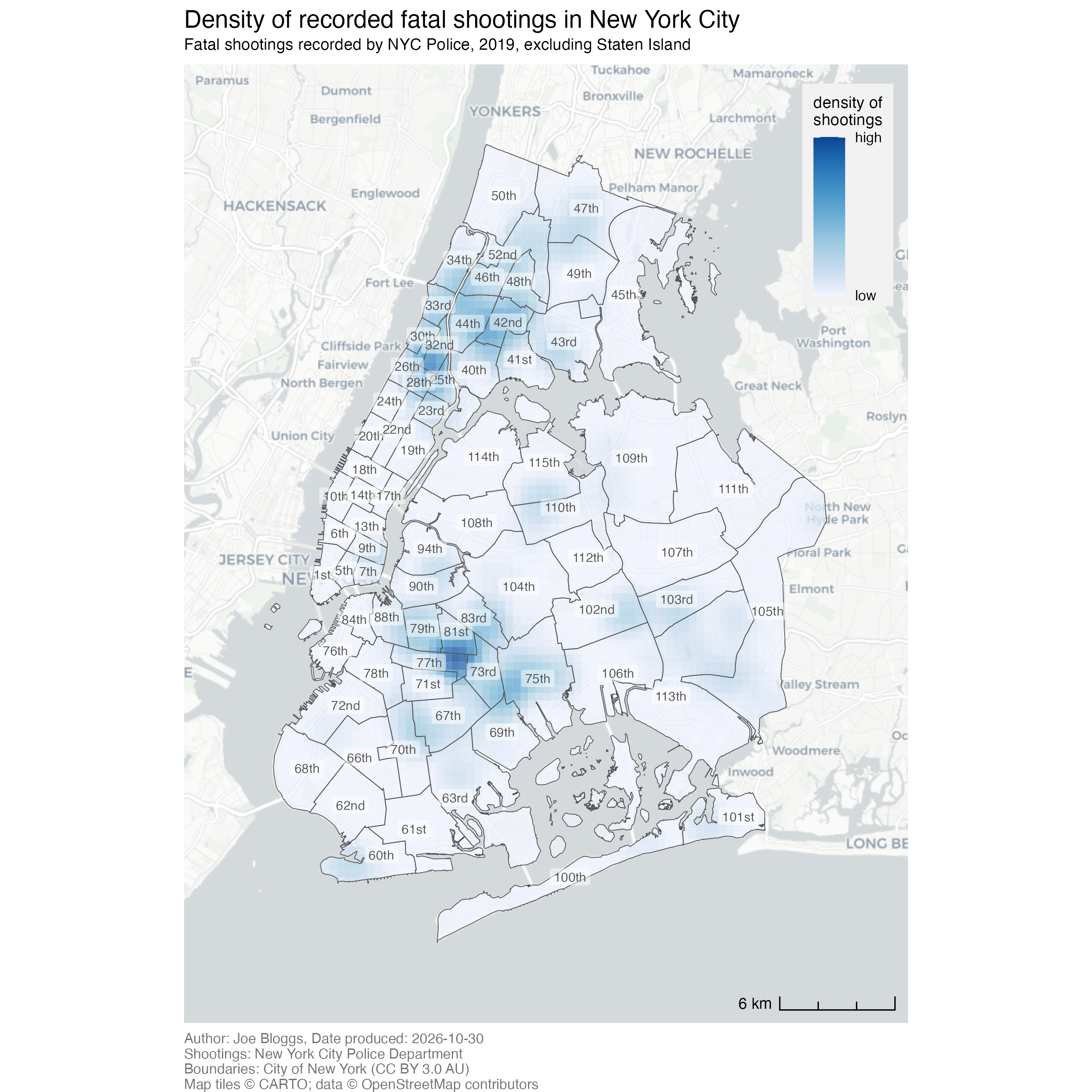
The finished map

<httr2_response>
GET https://mpjashby.github.io/crimemappingdata/nyc_shootings.csv
Status: 200 OK
Content-Type: text/csv
Body: On disk '/Users/mattashby/Documents/Crime Mapping Book/exercises/data/raw/nyc_shootings.csv' (69930 bytes)

<httr2_response>
GET https://mpjashby.github.io/crimemappingdata/nyc_precincts.gpkg
Status: 200 OK
Content-Type: application/octet-stream
Body: On disk '/Users/mattashby/Documents/Crime Mapping Book/exercises/data/raw/nyc_precincts.gpkg' (1769472 bytes)

Rows: 967 Columns: 6
── Column specification ────────────────────────────────────────────────────────
Delimiter: ","
chr  (1): boro
dbl  (3): incident_key, longitude, latitude
lgl  (1): murder
date (1): occur_date

ℹ Use `spec()` to retrieve the full column specification for this data.
ℹ Specify the column types or set `show_col_types = FALSE` to quiet this message.

Density map of recorded fatal shootings in New York City in 2019, excluding Staten Island. Darker blue indicates higher density. Police precinct boundaries and numbers are overlaid.

View the complete R script

# Map the density of recorded fatal shootings in NYC in 2019,
# excluding Staten Island.

# Note: both datasets will be harmonised to use EPSG:6538 for use with
# `hotspot_kde()`

## Load packages and data ------------------------------------------------------

# Load packages
pacman::p_load(ggspatial, here, httr2, sf, sfhotspot, tidyverse)

# Download the original data into the workspace
request("https://mpjashby.github.io/crimemappingdata/nyc_shootings.csv") |>
  req_perform(path = here("data", "raw", "nyc_shootings.csv"))
request("https://mpjashby.github.io/crimemappingdata/nyc_precincts.gpkg") |>
  req_perform(path = here("data", "raw", "nyc_precincts.gpkg"))

# Read local shootings data and select fatal shootings in 2019
shootings <- here("data", "raw", "nyc_shootings.csv") |>
  read_csv() |>
  janitor::clean_names() |>
  filter(murder == TRUE) |>
  st_as_sf(coords = c("longitude", "latitude"), crs = "EPSG:4326") |>
  st_transform("EPSG:6538")

# Load NYC police precincts data
precincts <- here("data", "raw", "nyc_precincts.gpkg") |>
  read_sf() |>
  janitor::clean_names() |>
  # Filter out precincts in Staten Island, since there are very few fatal
  # shootings there and it takes up a lot of space due to the position of Staten
  # Island relative to the rest of NYC
  filter(precinct <= 119) |>
  st_transform("EPSG:6538")


## Wrangle data ----------------------------------------------------------------

# Calculate KDE
shootings_kde <- shootings |>
  hotspot_kde(
    grid = hotspot_grid(precincts, cell_size = 400),
    bandwidth_adjust = 0.33,
    quiet = TRUE
  ) |>
  hotspot_clip(precincts, quiet = TRUE)


## Make map --------------------------------------------------------------------

shootings_map <- hotspot_map(
  shootings_kde,
  basemap_type = "cartolight",
  caption = str_glue(
    "Author: Joe Bloggs, Date produced: {today()}\n",
    "Shootings: New York City Police Department\n",
    "Boundaries: City of New York (CC BY 3.0 AU)"
  )
) +
  geom_sf(data = precincts, colour = "grey33", fill = NA) +
  geom_sf_label(
    aes(label = scales::ordinal(precinct)),
    data = precincts,
    alpha = 0.5,
    colour = "grey33",
    fill = "white",
    size = 2.5,
    linewidth = NA
  ) +
  annotation_scale(width_hint = 1 / 5, style = "ticks", location = "br") +
  labs(
    title = "Density of recorded fatal shootings in New York City",
    subtitle = "Fatal shootings recorded by NYC Police, 2019, excluding Staten Island",
    fill = "density of\nshootings"
  ) +
  theme(
    # We're going to overlay the legend on the map, so we should give the
    # legend a solid background
    legend.background = element_rect(colour = NA, fill = "#F2F2F2"),
    # Use the top-right corner of the legend as the anchor point for determining
    # its position
    legend.justification = c(1, 1),
    # Create a margin around the legend, since it has a solid background
    legend.margin = margin(6, 6, 6, 6),
    # Move the top-right corner of the legend to be very near the top-right
    # corner of the map
    legend.position = "inside",
    legend.position.inside = c(0.98, 0.98),
    # Make the legend and title smaller to reduce their visual prominence
    legend.text = element_text(size = rel(0.7)),
    legend.title = element_text(size = rel(0.8)),
    plot.subtitle = element_text(size = rel(0.8), margin = margin(3, 0, 6, 0)),
    plot.caption = element_text(colour = "grey45", size = rel(0.7), hjust = 0)
  )

# Save the finished map in the workspace output folder
ggsave(
  here("output", "nyc_fatal_shootings_2019.png"),
  plot = shootings_map,
  width = 210,
  height = 210,
  units = "mm"
)

Download the complete R script.

Step 1: Explain the script

1# Map the density of recorded fatal shootings in NYC in 2019,
# excluding Staten Island.

2# Note: both datasets will be harmonised to use EPSG:6538 for use with
# `hotspot_kde()`

1: It’s useful to start each script by explaining what it does. This makes it easier to find the right script if you need to revisit it later, for example to find a script that you can use as the basis for another script. In the case of data-analysis scripts, it’s useful to specify what the script is designed to produce, e.g. a map of a particular type (KDE) showing a particular crime type (fatal shootings) in a particular place (New York City) at a particular time (2019). See Organising code with comments.
2: To make it easier to combine the datasets later, we have decided to transform both spatial datasets to use the same co-ordinate reference system (CRS). Noting this policy decision here makes it easier to remember which CRS we are using when we are writing later parts of the script. See Transforming the coordinate reference system.

Step 2: Load packages

3## Load packages and data ------------------------------------------------------

# Load packages
4pacman::p_load(ggspatial, here, httr2, sf, sfhotspot, tidyverse)

3: Header comments divide the script into stages. These headings make it easier to find the part of a script you need once your scripts begin to get longer. See Organising code with comments.
4: pacman::p_load() loads the packages needed for this analysis, listed in alphabetical order with the tidyverse package last. ggspatial adds map elements such as scale bars; here allows us to specify where to find specific files; httr2 downloads data from the internet; sf handles spatial objects; sfhotspot calculates and maps density; and tidyverse provides tools for reading, selecting and plotting data. See Loading packages.

Step 3: Download the original data

# Download the original data into the workspace
5request("https://mpjashby.github.io/crimemappingdata/nyc_shootings.csv") |>
6  req_perform(path = here("data", "raw", "nyc_shootings.csv"))
request("https://mpjashby.github.io/crimemappingdata/nyc_precincts.gpkg") |>
  req_perform(path = here("data", "raw", "nyc_precincts.gpkg"))

5: request() specifies the URL of the file to download. The pipe operator (|>) passes that request to the next function. See Downloading and loading data; Stringing functions together.
6: req_perform() performs the download of the requested file. here() constructs a path to the data/raw folder in the workspace. The two downloads save the shootings CSV and precinct geopackage separately. This code assumes the workspace and folders have been set up as described in the book. See Keeping your files organised.

Step 4: Load and prepare the shootings data

# Read local shootings data and select fatal shootings in 2019
7shootings <- here("data", "raw", "nyc_shootings.csv") |>
8  read_csv() |>
9  janitor::clean_names() |>
10  filter(murder == TRUE) |>
11  st_as_sf(coords = c("longitude", "latitude"), crs = "EPSG:4326") |>
12  st_transform("EPSG:6538")

7: here() specifies which file we are going to load data from. <- stores the result of this whole pipeline as shootings, so later code can refer to it by name.
8: read_csv(), from readr, reads the local CSV file. See Loading CSV data; Naming objects.
9: janitor::clean_names(), from janitor, gives columns consistent names in snake_case. Naming the package before :: lets us use this function without loading the whole package. See Cleaning column names; Loading packages.
10: filter(), from dplyr, keeps rows that correspond to fatal shootings (murder == TRUE). TRUE is a logical value, which we denote by writing it in capitals without quotation marks. See Filtering rows; Map choices.
11: st_as_sf() tells R that the numbers in the longitude and latitude columns in the data represent points on the Earth’s surface. coords specifies which columns contain the x and y coordinates, in that order. crs = "EPSG:4326" identifies which coordinate reference system R should use to translate the numbers in those columns into geographic locations. See Converting data to an SF object.
12: st_transform() changes the coordinates to the projected CRS specified for this exercise. This prepares the points for density estimation and makes their CRS match the precinct boundaries. See Transforming the coordinate reference system.

Step 5: Load and prepare the precinct boundaries

# Load NYC police precincts data
13precincts <- here("data", "raw", "nyc_precincts.gpkg") |>
14  read_sf() |>
15  janitor::clean_names() |>
16  # Filter out precincts in Staten Island, since there are very few fatal
  # shootings there and it takes up a lot of space due to the position of Staten
  # Island relative to the rest of NYC
17  filter(precinct <= 119) |>
18  st_transform("EPSG:6538")

13: here() again specifies which file we are going to load data from. The result of this whole pipeline will be stored as precincts.
14: read_sf() reads the spatial file containing the precinct boundaries. Since this file is in a spatial data format (in this case, a geopackage), it includes the information R needs about the geometry and CRS, so we do not need to then use st_as_sf(). See Reading spatial data.
15: Clean the column names using the same convention as before.
16: At this point the code makes an important decision, to exclude Staten Island from the analysis. This is a judgement call on the part of the person who wrote this code – including Staten Island in the map would also have been a reasonable choice. The reason that this code excludes Staten Island is that has very few fatal shootings but is geographically large, so it would occupy a large proportion of the map if left included. Readers of crime analysis products such as crime maps are usually (although not always) interested in the areas with most crime, so excluding Staten Island allows for a more focused analysis of the areas with the highest crime rates. However, this depends very much on the intended audience of the map – if the intended audience was residents of Staten Island, for example, it would be more appropriate to include it. In any case, this is an important design choice so the comment explains the rationale behind it. Map choices.
17: filter(precinct <= 119) keeps only those precincts outside Staten Island, since the Staten Island precincts all have numbers 120 and above (we could find this out by mapping all the precinct numbers). See Filtering rows.
18: Transform the precinct boundaries to the same CRS as the shootings. Matching CRSs is often useful when using multiple spatial layers together.

Step 6: Calculate and clip the density layer

## Wrangle data ----------------------------------------------------------------

# Calculate KDE
19shootings_kde <- shootings |>
20  hotspot_kde(
21    grid = hotspot_grid(precincts, cell_size = 400),
22    bandwidth_adjust = 0.33,
23    quiet = TRUE
  ) |>
24  hotspot_clip(precincts, quiet = TRUE)

19: Start with the shootings object we created and specify that we will store the finished density layer as shootings_kde.
20: hotspot_kde() estimates the density of crimes in each cell in a grid. The arguments on the following lines control how it does this. See Mapping crime density.
21: hotspot_grid() uses the precinct boundaries to define the grid that will be used to estimate the density of shootings. cell_size = 400 sets the cells to 400 metres across. That’s larger than we would usually use for a city map, but New York City is very large so a KDE layer with a smaller cell size would take a very long time to estimate. See Specifying a grid for kernel density estimation; Fine-tuning cell size and bandwidth.
22: bandwidth_adjust = 0.33 reduces the default smoothing bandwidth, relative to the default bandwidth value. Setting a value of bandwidth_adjust below 1.0 reveals more local detail, but more detail is not automatically a better representation: bandwidth changes the patterns a reader sees.
23: quiet = TRUE suppresses the progress display that is produced by hotspot_kde(). That reduces the amount of text output in the R Console, but means you might miss important messages. If you are running a long-running analysis, you might want to set quiet = FALSE to see the progress.
24: hotspot_clip() clips the density layer to the area covered by the precincts layer. That makes sure we don’t inadvertently show incorrect density estimates for grid cells that are outside the area that we have crime data for. See Clipping map layers.

Step 7: Start the map and identify its sources

Create the base map and density layer, then record where the data came from.

## Make map --------------------------------------------------------------------

25shootings_map <- hotspot_map(
26  shootings_kde,
27  basemap_type = "cartolight",
28  caption = str_glue(
    "Author: Joe Bloggs, Date produced: {today()}\n",
    "Shootings: New York City Police Department\n",
    "Boundaries: City of New York (CC BY 3.0 AU)"
  )
29) +

25: Save the map as shootings_map. Keeping the map in an object lets us save the finished result in a subsequent step. See Creating and storing a map.
26: hotspot_map() uses the calculated density layer to start the map. See Mapping crime density.
27: The cartolight base map supplies geographic context with a relatively restrained appearance, helping the density layer remain prominent. See Base maps.
28: str_glue() from stringr allows us to combine multiple text values and R code into a single text value. The braces ({}) tell R to evaluate the code inside (today()) as R code rather than text, to insert the current date, while \n starts a new line. The caption credits the author and data providers, based on the information provided in the exercise instructions. Replace the example author name Joe Bloggs when producing your own map. See Using captions to add author and other information.
29: Note that this function finishes with a + operator because the same stack of functions continues in the next section. In the actual code this is a continuous stack of functions that make the map – they are just broken up here to explain each step.

Step 8: Add precinct boundaries and labels

30  geom_sf(data = precincts, colour = "grey33", fill = NA) +
31  geom_sf_label(
32    aes(label = scales::ordinal(precinct)),
33    data = precincts,
34    alpha = 0.5,
35    colour = "grey33",
36    fill = "white",
37    size = 2.5,
38    linewidth = NA
  ) +

30: geom_sf() overlays precinct boundaries on top of the density layer. The density layer should always be the most visually prominent layer on a density map, so it is important we display the precinct boundaries in a way that doesn’t obscure the density information. colour = "grey33" sets the outlines and fill = NA leaves the interiors unfilled so the density remains visible. See Adding more layers; Controlling aesthetics.
31: geom_sf_label() adds a label for each precinct. Again, it’s important that we don’t obscure the density layer when we do this, so several arguments are needed on subsequent lines to fine-tune the appearance of the labels.
32: aes() specifies which column in the precincts dataset to use for the label text. scales::ordinal(), from scales, converts numbers into forms such as “1st” and “2nd”, since that is how police precincts in New York City are typically referred to. See Formatting numbers using the scales package.
33: Specify which dataset to use for the precinct boundaries.
34: alpha = 0.5 makes the labels partly transparent, so they compete less with the density surface. See Visual hierarchy.
35: Use grey text (rather than the default black) to move the labels down the visual hierarchy.
36: A white background helps distinguish the label from the map beneath it, which improves readbility without moving the labels too far up the visual hierarchy since the backgrounds are semi-transparent.
37: Set a modest label-text size.
38: linewidth = NA removes the label border, reducing visual clutter.

Step 9: Add a scale bar and meaningful titles

39  annotation_scale(width_hint = 1 / 5, style = "ticks", location = "br") +
40  labs(
41    title = "Density of recorded fatal shootings in New York City",
42    subtitle = "Fatal shootings recorded by NYC Police, 2019, excluding Staten Island",
43    fill = "density of\nshootings"
  ) +

39: annotation_scale() from the ggspatial package adds a scale bar. width_hint = 1 / 5 suggests its width relative to the map, style = "ticks" chooses its appearance, and location = "br" places it at the bottom right. All these choices are made to make sure the scale bar appears at the bottom of the visual hierarchy. See Scale bars.
40: labs() supplies the map title, subtitle and fill-legend title. Note that we’ve already specified the map caption when we called hotspot_map(). See Supporting maps with words.
41: The title describes what is mapped. See Titles and subtitles.
42: The subtitle specifies the data provider, year and exclusion of Staten Island. Readers need this context to interpret the map correctly.
43: This line specifies the title for the map legend, which we can use to specify what the fill colours represent. Note that this title avoids any jargon like ‘kernel density’ or ‘KDE’ that might be unfamiliar to non-specialist readers. \n breaks the legend title over two lines. See Changing the legend title.

Step 10. Control the map layout

44  theme(
    # We're going to overlay the legend on the map, so we should give the
    # legend a solid background
45    legend.background = element_rect(colour = NA, fill = "#F2F2F2"),
    # Use the top-right corner of the legend as the anchor point for determining
    # its position
46    legend.justification = c(1, 1),
    # Create a margin around the legend, since it has a solid background
47    legend.margin = margin(6, 6, 6, 6),
    # Move the top-right corner of the legend to be very near the top-right
    # corner of the map
48    legend.position = "inside",
49    legend.position.inside = c(0.98, 0.98),
    # Make the legend and title smaller to reduce their visual prominence
50    legend.text = element_text(size = rel(0.7)),
    legend.title = element_text(size = rel(0.8)),
51    plot.subtitle = element_text(size = rel(0.8), margin = margin(3, 0, 6, 0)),
52    plot.caption = element_text(colour = "grey45", size = rel(0.7), hjust = 0)
  )

44: theme(), from ggplot2, controls the aspects of the plot that are not controlled by the data. It can change the position of the legend, text sizes, background colours and the appearance of other map elements. In this case we will use this to move the legend onto a part of the map area that is not covered by the date. Doing that means the map area can expand to fill the space that would otherwise be occupied by the legend, giving the map area slightly more space. See Changing the appearance of titles and captions; Visual hierarchy.
45: Give the legend a solid background so it can be seen on top of the base map.
46: Use the top-right corner of the legend as the anchor for positioning it.
47: Add some space between the legend contents and the edge of the solid background we’ve just created.
48: Place the legend inside the map to leave more room for the geographic information.
49: Position the legend near the top right. The values run from 0 to 1 across and up the map area, so c(0.98, 0.98) represents a location almost at the top-right corner of the map.
50: rel() sets text size relative to the theme’s base text size. Reduce legend text and its title so they support the map without dominating it.
51: Adjust the subtitle size and the spacing around it.
52: Make the caption smaller and grey. hjust = 0 aligns it to the left. The closing brackets complete theme() and the map expression. See Using captions to add author and other information.

Step 11: Save the finished map

# Save the finished map in the workspace output folder
53ggsave(
54  here("output", "nyc_fatal_shootings_2019.png"),
55  plot = shootings_map,
56  width = 210,
57  height = 210,
58  units = "mm"
)

53: ggsave() writes the map to a file on your computer, using the settings specified on the following lines. See Saving maps.
54: Specify where on your computer the map should be saved, relative to the crime_mapping workspace folder. The .png extension specifies that the file should be saved in PNG format. See Keeping your files organised.
55: Specify the object containing the map to save. See Creating and storing a map.
56: Set the output width to 210 mm.
57: Set the height to 210 mm as well, making the overall image square.
58: Specify that the dimensions are in millimetres. The finished image is 210 × 210 mm.