Mapping stalking rates in Queensland: specimen answer

Return to the exercise.

This document walks through a specimen answer to this exercise. Read each code section and its numbered explanations below. Select the number at the start of each explanation to highlight the line of code that explanation relates to.

In R, like in many programming languages, there is usually more than one way to complete a task. This code shows one way to complete this exercise. There are other ways to organise this code that are equally good and achieve the same result, but the code below tries to balance making the code efficient with making it easy to read. If your code is different from the code here, read through the notes below the answer and use those to decide whether you prefer your own approach or the specimen answer below. You can also use the notes to improve your own code.

The specimen answer expects your computer to be set up as outlined in the book.

The online textbook sets out how to install the software you need for crime mapping with R and set up your computer to store files in particular places. The specimen answer below assumes that you have followed those instructions and that your computer is set up as described in the book. If you have not done so, the code in the specimen answer may not run correctly.

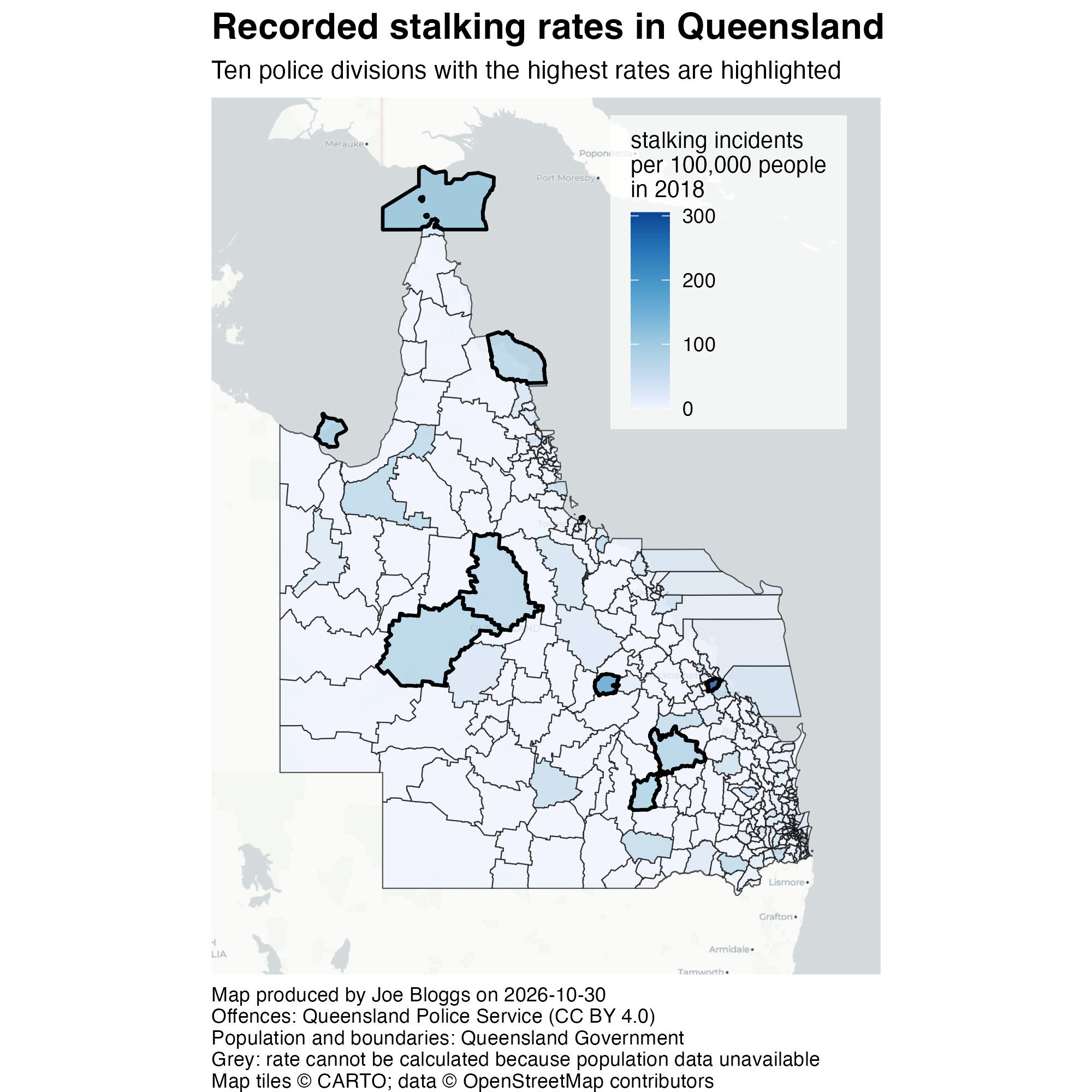
The finished map

<httr2_response>
GET https://mpjashby.github.io/crimemappingdata/qld_stalking.xlsx
Status: 200 OK
Content-Type: application/vnd.openxmlformats-officedocument.spreadsheetml.sheet
Body: On disk '/Users/mattashby/Documents/Crime Mapping Book/exercises/data/raw/qld_stalking.xlsx' (104030 bytes)

<httr2_response>
GET https://mpjashby.github.io/crimemappingdata/qld_population.csv.gz
Status: 200 OK
Content-Type: application/gzip
Body: On disk '/Users/mattashby/Documents/Crime Mapping Book/exercises/data/raw/qld_population.csv.gz' (2867 bytes)

<httr2_response>
GET https://mpjashby.github.io/crimemappingdata/qld_police_divisions.gpkg
Status: 200 OK
Content-Type: application/octet-stream
Body: On disk '/Users/mattashby/Documents/Crime Mapping Book/exercises/data/raw/qld_police_divisions.gpkg' (8941568 bytes)

Rows: 334 Columns: 2
── Column specification ────────────────────────────────────────────────────────
Delimiter: ","
chr (1): police_division
dbl (1): population

ℹ Use `spec()` to retrieve the full column specification for this data.
ℹ Specify the column types or set `show_col_types = FALSE` to quiet this message.

Choropleth map of recorded stalking incidents per 100,000 residents in Queensland police divisions in 2018. Darker blue indicates higher rates. The ten divisions with the highest rates are outlined; grey indicates a missing rate.

View the complete R script

# Map recorded stalking incidents per 100,000 residents in Queensland in 2018.

# Load packages
pacman::p_load(here, httr2, sf, sfhotspot, tidyverse)


# Load data --------------------------------------------------------------------

# Download the original data into the workspace
request("https://mpjashby.github.io/crimemappingdata/qld_stalking.xlsx") |>
  req_perform(path = here("data", "raw", "qld_stalking.xlsx"))
request("https://mpjashby.github.io/crimemappingdata/qld_population.csv.gz") |>
  req_perform(path = here("data", "raw", "qld_population.csv.gz"))
request(
  "https://mpjashby.github.io/crimemappingdata/qld_police_divisions.gpkg"
) |>
  req_perform(path = here("data", "raw", "qld_police_divisions.gpkg"))

# Read local data and select stalking counts for 2018
# No need to specify the `sheet` argument in `read_excel()` because the Excel
# file only has one sheet
stalking <- here("data", "raw", "qld_stalking.xlsx") |>
  readxl::read_excel() |>
  filter(year == 2018)
population <- here("data", "raw", "qld_population.csv.gz") |>
  read_csv()
divisions <- here("data", "raw", "qld_police_divisions.gpkg") |>
  read_sf()


# Wrangle data -----------------------------------------------------------------

# Join data and calculate rate
stalking_rate <- divisions |>
  left_join(population, by = join_by(division == police_division)) |>
  left_join(stalking, by = join_by(division)) |>
  mutate(rate = stalking / population * 100000)

# Pimpama has no matching population, so its rate remains NA.
# Keep it on the map in grey rather than treating missing data as zero.

# Find divisions with highest stalking rate
stalking_rate_highest <- slice_max(
  stalking_rate,
  rate,
  n = 10,
  with_ties = FALSE
)


# Create map -------------------------------------------------------------------

stalking_map <- hotspot_map(
  stalking_rate,
  mapping = aes(fill = rate),
  basemap_type = "cartolight",
  caption = str_glue(
    "Map produced by Joe Bloggs on {today()}\n",
    "Offences: Queensland Police Service (CC BY 4.0)\n",
    "Population and boundaries: Queensland Government\n",
    "Grey: rate cannot be calculated because population data unavailable"
  ),
  alpha = 0.75,
  linewidth = 0.25
) +
  # Add thicker boundaries for 10 divisions with highest rates
  geom_sf(
    data = stalking_rate_highest,
    colour = "black",
    fill = NA,
    linewidth = 0.75
  ) +
  scale_fill_distiller(direction = 1) +
  labs(
    title = "Recorded stalking rates in Queensland",
    subtitle = str_glue(
      "Ten police divisions with the highest rates are highlighted"
    ),
    fill = "stalking incidents\nper 100,000 people\nin 2018"
  ) +
  theme(
    # Slightly lower the legend in the visual hierarchy by giving it a
    # background that is white and semi-transparent
    legend.background = element_rect(colour = NA, fill = rgb(1, 1, 1, 0.75)),
    # Base legend position on the top-right corner of the legend, which makes
    # moving the legend to the top-right corner easier
    legend.justification = c(1, 1),
    # Add some padding around the legend
    legend.margin = margin(6, 9, 9, 9),
    # Move the legend almost to the top-right corner of the map, since this is
    # the area of the map with no content in it
    legend.position = "inside",
    legend.position.inside = c(0.95, 0.98),
    # Make the legend title slightly smaller, again reducing its prominence
    legend.title = element_text(size = 10),
    # Left-align the caption
    plot.caption = element_text(hjust = 0),
    # Add some space above and below the plot subtitle
    plot.subtitle = element_text(margin = margin(6, 0, 6, 0)),
    # Make the plot title larger and bold to move it up the visual hierarchy
    plot.title = element_text(face = "bold", size = 16)
  )


# Save map ---------------------------------------------------------------------

# Create map that is 2000px x 2000px
ggsave(
  filename = here("output", "queensland_stalking_rate_map_2018.jpg"),
  plot = stalking_map,
  width = 2000,
  height = 2000,
  units = "px"
)

Download the complete R script.

Step 1: Explain the script

1# Map recorded stalking incidents per 100,000 residents in Queensland in 2018.

1: Explain that the script maps recorded stalking incidents per 100,000 residents in Queensland in 2018. It is important to note that this map shows a rate, not a count. See Organising code with comments.

Step 2: Load packages

# Load packages
2pacman::p_load(here, httr2, sf, sfhotspot, tidyverse)

2: pacman::p_load() loads the packages needed for this analysis, listed in alphabetical order with the tidyverse package last. here allows us to specify where to find files in the workspace; httr2 downloads data from the internet; sf handles spatial objects; sfhotspot creates crime maps and estimates density; tidyverse provides tools for reading, wrangling and plotting data. Loading packages at the start makes it easy to check which tools the script needs. See Loading packages.

Step 3: Download the original data

# Load data --------------------------------------------------------------------

# Download the original data into the workspace
3request("https://mpjashby.github.io/crimemappingdata/qld_stalking.xlsx") |>
4  req_perform(path = here("data", "raw", "qld_stalking.xlsx"))
request("https://mpjashby.github.io/crimemappingdata/qld_population.csv.gz") |>
  req_perform(path = here("data", "raw", "qld_population.csv.gz"))
request(
  "https://mpjashby.github.io/crimemappingdata/qld_police_divisions.gpkg"
) |>
  req_perform(path = here("data", "raw", "qld_police_divisions.gpkg"))

3: request() specifies the URL of the file to download. The pipe operator (|>) passes that request to the next function. Download the stalking counts, population counts and police division boundaries separately. All three are needed: the boundaries identify the areas, and the two sets of counts provide the numerator and denominator of the rate. See Downloading and loading data; Stringing functions together.
4: req_perform() performs the download set up by the corresponding call to request(). here() specifies where the original file should be saved, relative to the crime_mapping workspace. Keeping an unchanged copy of the original data in data/raw means we can return to it if we make a mistake while wrangling the data. See Keeping your files organised.

Step 4: Read the three datasets

# Read local data and select stalking counts for 2018
5# No need to specify the `sheet` argument in `read_excel()` because the Excel
# file only has one sheet
6stalking <- here("data", "raw", "qld_stalking.xlsx") |>
7  readxl::read_excel() |>
8  filter(year == 2018)
9population <- here("data", "raw", "qld_population.csv.gz") |>
10  read_csv()
11divisions <- here("data", "raw", "qld_police_divisions.gpkg") |>
12  read_sf()

5: The comment explains why the Excel-reading function below has no sheet argument: the supplied file has only one sheet. Comments can record decisions as well as describe actions. See Organising code with comments.
6: Locate the Excel workbook with here() and store the finished pipeline as stalking. See Keeping your files organised.
7: read_excel() from readxl reads the workbook. Using :: lets us use this function without loading the whole package. See Loading Excel data.
8: filter() from dplyr keeps only rows where year equals 2018. This prevents counts from different years being joined to the same division later. See Filtering rows.
9: here() locates the downloaded population file within the workspace. The pipe passes this path to read_csv().
10: read_csv() from readr reads the compressed population CSV without a separate decompression step. These population counts are from 2016, so the rate will use an earlier population than the 2018 offences. See Loading CSV data; Choosing a population measure.
11: here() locates the downloaded police division boundaries within the workspace. The pipe passes this path to read_sf().
12: read_sf() reads the geopackage as a spatial object. Its geometry and CRS information are already in the file. These boundaries are from 2022; reading them does not make them the boundaries that existed in 2018. See Reading spatial data.

Step 5: Join the datasets and calculate rates

# Wrangle data -----------------------------------------------------------------

# Join data and calculate rate
13stalking_rate <- divisions |>
14  left_join(population, by = join_by(division == police_division)) |>
15  left_join(stalking, by = join_by(division)) |>
16  mutate(rate = stalking / population * 100000)

17# Pimpama has no matching population, so its rate remains NA.
# Keep it on the map in grey rather than treating missing data as zero.

13: Start with divisions and store the finished result as stalking_rate. Keeping the boundaries on the left of the joins means that divisions can remain on the map even when a count is missing. See Combining datasets.
14: Join each division to its population using division in the boundary data and police_division in the population data. join_by() specifies which values must match; the two columns do not have to share a name.
15: Join the 2018 stalking counts using the division column, which has the same name in both datasets.
16: mutate() calculates a new column called rate: divide stalking incidents by the population and multiply by 100,000. This lets us compare areas with different population sizes. See Calculating crime rates; Transforming values.
17: The Pimpama division has no matching population figure, so the value for the rate column is NA (the way R represents missing values) because it’s not possible to calculate a rate without both stalking incidents and population data. We keep that division on the map, show the missing data using a grey fill and explain the grey fill in the caption. See Missing values.

Step 6: Find the ten highest rates

This step implements the optional challenge in the exercise. It is useful to keep these selected divisions in a separate object, so that they can be added as extra map layers.

# Find divisions with highest stalking rate
18stalking_rate_highest <- slice_max(
  stalking_rate, 
  rate, 
  n = 10, 
  with_ties = FALSE
)

18: Use slice_max() to keep only the ten divisions with the highest stalking rates. with_ties = FALSE limits the result to ten even if rates are tied. Store the result in a new object called stalking_rate_highest.

Step 7: Start the map and identify its sources

# Create map -------------------------------------------------------------------

19stalking_map <- hotspot_map(
20  stalking_rate,
21  mapping = aes(fill = rate),
22  basemap_type = "cartolight",
23  caption = str_glue(
    "Map produced by Joe Bloggs on {lubridate::today()}\n",
    "Offences: Queensland Police Service (CC BY 4.0)\n",
    "Population and boundaries: Queensland Government\n",
    "Grey: rate cannot be calculated because population data unavailable"
  ),
24  alpha = 0.75,
25  linewidth = 0.25
26) +

19: Store the finished map as stalking_map, so it can be saved to a file in the final step. See Creating and storing a map.
20: Use all divisions with their calculated rates as the basis of hotspot_map().
21: aes(fill = rate) tells hotspot_map() to fill each division according to its rate. We need to specify this relationship ourselves because stalking_rate was not an object created by one of the hotspot_*() family of functions. See Controlling fill colours when mapping rates.
22: Use a light cartolight base map to provide geographic context while not overwhelming the map with too much detail or distracting from the data layer. See Base maps.
23: str_glue() combines the author, date and data sources into the caption. today() from the lubridate package inserts the date the script runs. The final line explains that grey means the population needed for a rate is unavailable. Replace Joe Bloggs with your own name. See Using captions to add author and other information.
24: Make the division fills partly transparent so that readers can still see the base map beneath them. See Controlling aesthetics.
25: Use thin outlines for the main divisions. The highlighted divisions added next will have thicker outlines, so they stand out without the whole map becoming a mass of boundary lines. See Visual hierarchy.
26: The + operator continues the same map expression in the following section. In the complete script these layers form one continuous stack.

Step 8: Highlight the ten selected divisions

  # Add thicker boundaries for 10 divisions with highest rates
27  geom_sf(
28    data = stalking_rate_highest,
29    colour = "black",
30    fill = NA,
31    linewidth = 0.75
  ) +

27: geom_sf() adds an extra boundary layer over the rate map. See Adding more layers.
28: Use only stalking_rate_highest for this layer, rather than outlining every division again.
29: Use black outlines so the selected divisions stand out from the other boundaries. See Visual hierarchy.
30: Leave the interiors unfilled with fill = NA, preserving the rate colours beneath them.
31: Use a width of 0.75, compared with 0.25 for the main layer, to make the selected outlines more prominent.

Step 9: Specify the colours and map text

32  scale_fill_distiller(direction = 1) +
33  labs(
34    title = "Recorded stalking rates in Queensland",
35    subtitle = str_glue(
      "Ten police divisions with the highest rates are highlighted"
    ),
36    fill = "stalking incidents\nper 100,000 people\nin 2018"
  ) +

32: scale_fill_distiller(direction = 1) uses the default sequential palette with higher rates shown in darker colours. This makes the highest rates more visually prominent. See Controlling fill colours when mapping rates.
33: labs() supplies the title, subtitle and legend title. See Titles and subtitles.
34: Identify the subject and place: recorded stalking rates in Queensland.
35: Explain why ten divisions have been highlighted. str_glue() is retained here, although a plain text string would also work because this subtitle contains no inserted values.
36: State the rate units and year in the legend title. Whenever you map a rate, it is important to specify how the rate was calculated. In this case, the rate is the number of stalking incidents per 100,000 people in 2018. Stating that makes for a much more informative legend title than one that said simply “stalking rate” or similar. The line breaks (\n) keep the title narrow enough to fit beside the colour bar. See Changing the legend title.

Step 10: Control the map layout

37  theme(
    # Slightly lower the legend in the visual hierarchy by giving it a
    # background that is white and semi-transparent
38    legend.background = element_rect(colour = NA, fill = rgb(1, 1, 1, 0.75)),
    # Base legend position on the top-right corner of the legend, which makes
    # moving the legend to the top-right corner easier
39    legend.justification = c(1, 1),
    # Add some padding around the legend
40    legend.margin = margin(6, 9, 9, 9),
    # Move the legend almost to the top-right corner of the map, since this is
    # the area of the map with no content in it
41    legend.position = "inside",
42    legend.position.inside = c(0.95, 0.98),
    # Make the legend title slightly smaller, again reducing its prominence
43    legend.title = element_text(size = 10),
    # Left-align the caption
44    plot.caption = element_text(hjust = 0),
    # Add some space above and below the plot subtitle
45    plot.subtitle = element_text(margin = margin(6, 0, 6, 0)),
    # Make the plot title larger and bold to move it up the visual hierarchy
46    plot.title = element_text(face = "bold", size = 16)
  )

37: theme() from ggplot2 adjusts supporting elements of the map. The following choices make the legend readable while leaving more space for the geography. See Changing the appearance of titles and captions; Visual hierarchy.
38: element_rect() gives the legend no border and a partly transparent white background. rgb(1, 1, 1, 0.75) specifies white with opacity 0.75.
39: Use the top-right corner of the legend as the anchor when positioning it.
40: Add padding around the legend contents to separate them from the map beneath.
41: Place the legend inside the map area.
42: Position it near the top right. Values close to 1 mean close to the right and top edges; this uses an area with little map content.
43: Use a slightly smaller legend title to reduce its prominence.
44: Left-align the caption using hjust = 0. See Using captions to add author and other information.
45: Add some space above and below the subtitle.
46: Make the title larger and bold so that it appears higher in the visual hierarchy. The closing brackets finish the map expression.

Step 11: Save the finished map

# Save map ---------------------------------------------------------------------

# Create map that is 2000px x 2000px
47ggsave(
48  filename = here("output", "queensland_stalking_rate_map_2018.jpg"),
49  plot = stalking_map,
50  width = 2000,
  height = 2000,
51  units = "px"
)

47: ggsave() from ggplot2 writes the map to a file on your computer, using the settings on the following lines. See Saving maps.
48: Specify where the map should be saved, relative to the workspace. The file name queensland_stalking_rate_map_2018.jpg also specifies the image format. See Keeping your files organised.
49: Specify the map object to save, in this case stalking_map. This avoids relying on whichever plot was displayed most recently. See Creating and storing a map.
50: Set the width and height to 2000 pixels.
51: Specify that the dimensions are measured in pixels (px).