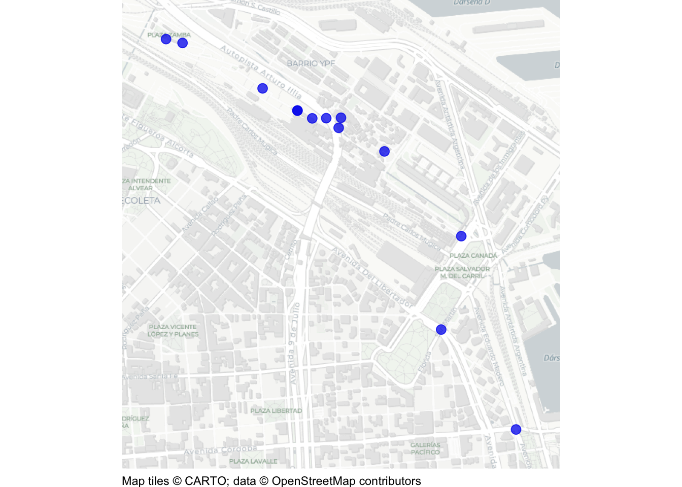
Mapping homicides in Retiro: specimen answer

Return to the exercise.

This document walks through a specimen answer to this exercise. Read each code section and its numbered explanations below. Select the number at the start of each explanation to highlight the line of code that explanation relates to.

In R, like in many programming languages, there is usually more than one way to complete a task. This code shows one way to complete this exercise. There are other ways to organise this code that are equally good and achieve the same result, but the code below tries to balance making the code efficient with making it easy to read. If your code is different from the code here, read through the notes below the answer and use those to decide whether you prefer your own approach or the specimen answer below. You can also use the notes to improve your own code.

The specimen answer expects your computer to be set up as outlined in the book.

The online textbook sets out how to install the software you need for crime mapping with R and set up your computer to store files in particular places. The specimen answer below assumes that you have followed those instructions and that your computer is set up as described in the book. If you have not done so, the code in the specimen answer may not run correctly.

The finished map

<httr2_response>
GET https://mpjashby.github.io/crimemappingdata/retiro_homicides.csv
Status: 200 OK
Content-Type: text/csv
Body: On disk '/Users/mattashby/Documents/Crime Mapping Book/exercises/data/raw/retiro_homicides.csv' (710 bytes)

Rows: 13 Columns: 4
── Column specification ────────────────────────────────────────────────────────
Delimiter: ","
dbl  (3): id_mapa, longitud, latitud
dttm (1): fecha

ℹ Use `spec()` to retrieve the full column specification for this data.
ℹ Specify the column types or set `show_col_types = FALSE` to quiet this message.

Point map of recorded homicides in the Retiro neighbourhood of Buenos Aires in 2023. Blue points mark incident locations on a light street base map.

View the complete R script

# Map recorded homicides in the Retiro neighbourhood of Buenos Aires in 2023.

# Load packages
pacman::p_load(here, httr2, sf, sfhotspot, tidyverse)

# Download the original data and keep a local copy
request("https://mpjashby.github.io/crimemappingdata/retiro_homicides.csv") |>
  req_perform(path = here("data", "raw", "retiro_homicides.csv"))

# Read data
homicides <- here("data", "raw", "retiro_homicides.csv") |>
  read_csv()

# Convert longitude and latitude to a spatial object
homicides_sf <- st_as_sf(
  homicides,
  coords = c("longitud", "latitud"),
  crs = "EPSG:4326"
)

# Transform to a projected coordinate reference system suitable for Buenos Aires
homicides_sf_trans <- st_transform(homicides_sf, crs = "EPSG:5348")

# Display the map
hotspot_map(
  homicides_sf_trans,
  basemap_type = "cartolight",
  colour = "blue2",
  size = 3
)

Download the complete R script.

Step 1: Explain the script

1# Map recorded homicides in the Retiro neighbourhood of Buenos Aires in 2023.

1: Start by specifying what the script is designed to produce: a map of recorded homicides in Retiro in 2023. This makes it easier to identify the script if we want to revisit it or use it as the basis for another analysis. See Organising code with comments.

Step 2: Load packages

# Load packages
2pacman::p_load(here, httr2, sf, sfhotspot, tidyverse)

2: pacman::p_load() loads the packages needed for this analysis, listed in alphabetical order with the tidyverse package last. here allows us to specify where to find files in the workspace; httr2 downloads data from the internet; sf handles spatial objects; sfhotspot makes it easy to make crime maps; tidyverse provides tools for reading, wrangling and plotting data. Loading packages at the start makes it easy to check which tools the script needs. See Loading packages.

Step 3: Download the original data

# Download the original data and keep a local copy
3request("https://mpjashby.github.io/crimemappingdata/retiro_homicides.csv") |>
4  req_perform(path = here("data", "raw", "retiro_homicides.csv"))

3: request() specifies the URL of the file to download. The pipe operator (|>) passes that request to the next function. The supplied CSV already contains the recorded homicides for the place and year requested in the exercise, so we do not need to download a larger dataset and filter it. See Downloading and loading data; Stringing functions together.
4: req_perform() performs the download that was set up by request(). here() specifies where the original file should be saved, relative to the crime_mapping workspace. Keeping an unchanged copy of the original data in data/raw means we can return to it if we make a mistake while wrangling the data. See Keeping your files organised.

Step 4: Read the downloaded data

# Read data
5homicides <- here("data", "raw", "retiro_homicides.csv") |>
6  read_csv()

5: here() specifies the path to the downloaded CSV file within the workspace. The pipe (|>) passes this path to read_csv().
6: read_csv() from readr reads the local CSV file from the path passed through the pipe. <- stores the result as homicides, so that we can refer to those records in the following steps. See Loading CSV data; Naming objects.

Step 5: Convert the data to a spatial object

# Convert longitude and latitude to a spatial object
7homicides_sf <- st_as_sf(
8  homicides,
9  coords = c("longitud", "latitud"),
10  crs = "EPSG:4326"
)

7: st_as_sf() converts an ordinary object into a spatial object which specifies how the coordinates in the data correspond to locations of the earth, and stores the result as homicides_sf. The arguments below tell R how to interpret the coordinate columns. See Converting data to an SF object.
8: Use the records in homicides as the basis of the new spatial object.
9: The coordinate columns have Spanish names. longitud contains the x coordinates and latitud contains the y coordinates. We must use the actual column names, in that order, rather than translating them into English.
10: crs = "EPSG:4326" (CRS means coordinate reference system) describes the existing coordinates as longitude and latitude. Assigning this CRS tells R how to translate the numbers in those columns to geographic locations. It’s worth noting here that the crs argument in st_as_sf() describes the coordinate system that the data uses – in the next step we will change (transform) that coordinate system.

Step 6: Transform the coordinates

# Transform to a projected coordinate reference system suitable for Buenos Aires
11homicides_sf_trans <- st_transform(homicides_sf, crs = "EPSG:5348")

11: st_transform() changes the data so that the coordinates are specified using the POSGAR 2007 / Argentina 6 coordinate reference system, a projected CRS that is suitable for mapping Buenos Aires. The result is stored as homicides_sf_trans. Remember: st_as_sf() described the coordinates already in the file, while st_transform() changes them into a different system. See Transforming the coordinate reference system.

Step 7: Draw the map

# Display the map
12hotspot_map(
13  homicides_sf_trans,
14  basemap_type = "cartolight",
15  colour = "blue2",
16  size = 3
)

12: hotspot_map() draws the spatial points over a base map. Note that the result of this function is not stored in an object using <-, so running it causes the result (in this case, the map) to be displayed directly on the screen. See Drawing the map.
13: Specify which object contains the data that we want to map. By this point we’ve created several objects, so make sure the code here refers to the correct object: homicides_sf_trans, not homicides or homicides_sf.
14: Choose the light cartolight style of base map to provide local context without visually competing with the points showing the homicides. See Base maps.
15: Blue points contrast with the light base map, making it easier to identify where the homicides happened. See Visual hierarchy.
16: Make the points larger than the default, since we want the incidents to be easy to see over the base map. See Controlling aesthetics.