Mapping homicides in the São Paulo region: specimen answer

Return to the exercise.

This document walks through a specimen answer to this exercise. Read each code section and its numbered explanations below. Select the number at the start of each explanation to highlight the line of code that explanation relates to.

In R, like in many programming languages, there is usually more than one way to complete a task. This code shows one way to complete this exercise. There are other ways to organise this code that are equally good and achieve the same result, but the code below tries to balance making the code efficient with making it easy to read. If your code is different from the code here, read through the notes below the answer and use those to decide whether you prefer your own approach or the specimen answer below. You can also use the notes to improve your own code.

WarningThe specimen answer expects your computer to be set up as outlined in the book.

The online textbook sets out how to install the software you need for crime mapping with R and set up your computer to store files in particular places. The specimen answer below assumes that you have followed those instructions and that your computer is set up as described in the book. If you have not done so, the code in the specimen answer may not run correctly.

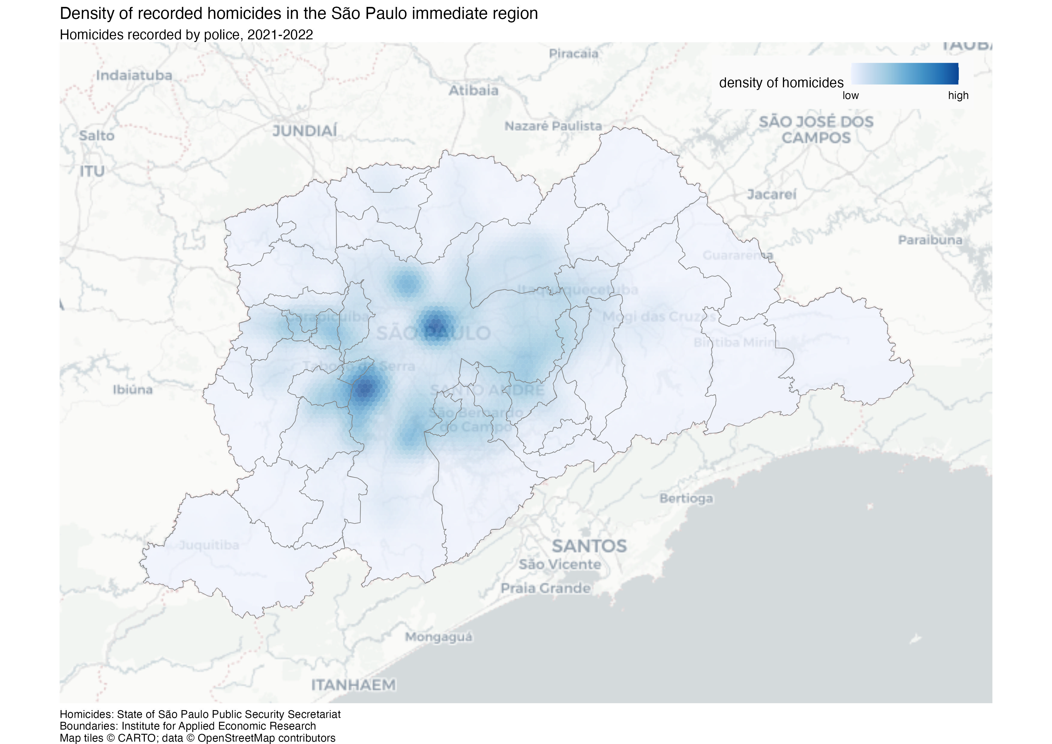
The finished map

<httr2_response>
GET https://mpjashby.github.io/crimemappingdata/sao_paulo_homicides.xlsx
Status: 200 OK
Content-Type: application/vnd.openxmlformats-officedocument.spreadsheetml.sheet
Body: On disk '/Users/mattashby/Documents/Crime Mapping Book/exercises/data/raw/sao_paulo_homicides.xlsx' (287101 bytes)

<httr2_response>
GET https://mpjashby.github.io/crimemappingdata/sao_paulo_muni.geojson
Status: 200 OK
Content-Type: application/geo+json
Body: On disk '/Users/mattashby/Documents/Crime Mapping Book/exercises/data/raw/sao_paulo_muni.geojson' (308430 bytes)

NoteView the complete R script

# This script creates a density map of homicides in São Paulo, Brazil, from 2021
# to 2022

# Load packages ----
pacman::p_load(here, httr2, sf, sfhotspot, tidyverse)


# Load data ----

# Download the original data into the workspace
request(
  "https://mpjashby.github.io/crimemappingdata/sao_paulo_homicides.xlsx"
) |>
  req_perform(path = here("data", "raw", "sao_paulo_homicides.xlsx"))
request("https://mpjashby.github.io/crimemappingdata/sao_paulo_muni.geojson") |>
  req_perform(path = here("data", "raw", "sao_paulo_muni.geojson"))

homicides <- here("data", "raw", "sao_paulo_homicides.xlsx") |>
  # Read Excel file -- there is only one sheet so we won't need to specify
  readxl::read_excel() |>
  # Convert names to snake_case
  janitor::clean_names() |>
  # Keep only homicides in 2021 and 2022
  filter(between(year, 2021, 2022)) |>
  # Convert to an SF object
  st_as_sf(coords = c("longitude", "latitude"), crs = "EPSG:4326") |>
  # Convert to a CRS that uses metres
  st_transform("EPSG:5538")

# Load boundary data
muni <- here("data", "raw", "sao_paulo_muni.geojson") |>
  read_sf() |>
  # Convert names to snake_case
  janitor::clean_names() |>
  # Convert to a CRS that uses metres
  st_transform("EPSG:5538")


# Wrangle data ----

# Create KDE layer
homicides_kde <- homicides |>
  # Estimate density of homicides. São Paulo is very large, so use a larger
  # cell size than for most cities.
  hotspot_kde(
    grid = hotspot_grid(muni, cell_size = 1000, grid_type = "hex"),
    bandwidth_adjust = 0.33,
    quiet = TRUE
  ) |>
  # Clip the density layer to the area for which we have data
  hotspot_clip(muni, quiet = TRUE)


# Map data ----

# Create map
homicide_map <- hotspot_map(
  homicides_kde,
  basemap_type = "cartolight",
  caption = str_glue(
    "Homicides: State of São Paulo Public Security Secretariat\n",
    "Boundaries: Institute for Applied Economic Research"
  )
) +
  geom_sf(data = muni, colour = "grey50", fill = NA) +
  labs(
    title = "Density of recorded homicides in the São Paulo immediate region",
    subtitle = "Homicides recorded by police, 2021-2022",
    fill = "density of homicides"
  ) +
  # Remove unnecessary map elements
  theme(
    # Put a box around the legend to make it easier to read
    legend.background = element_rect(colour = NA, fill = "grey98"),
    # Since the map is wider than it is tall, change the legend to correspond
    legend.direction = "horizontal",
    # Make the legend expand relative to its top-right corner
    legend.justification = c(1, 1),
    # Add some space around the legend to make it easier to read
    legend.margin = margin(6, 12, 6, 6),
    # Move the legend inside the map area
    legend.position = "inside",
    # Position the legend in the top-right corner of the map
    legend.position.inside = c(0.98, 0.98)
  )

# Save map
ggsave(
  filename = here("output", "sao_paulo_homicide_2021_22.jpg"),
  plot = homicide_map,
  width = 297,
  height = 210,
  units = "mm"
)

Download the complete R script.

Step 1: Explain the script

1# This script creates a density map of homicides in São Paulo, Brazil, from 2021
# to 2022

1

Explain that the script creates a density map of homicides in São Paulo in 2021 and 2022. Giving the crime type, place and period makes the purpose clear when we return to the script later. See Organising code with comments.

Step 2: Load packages

# Load packages ----
2pacman::p_load(here, httr2, sf, sfhotspot, tidyverse)

2

pacman::p_load() loads the packages needed for this analysis, listed in alphabetical order with the tidyverse package last. here allows us to specify where to find files in the workspace; httr2 downloads data from the internet; sf handles spatial objects; sfhotspot creates crime maps and estimates density; tidyverse provides tools for reading, wrangling and plotting data. Loading packages at the start makes it easy to check which tools the script needs. See Loading packages.

Step 3: Download the original data

# Load data ----

# Download the original data into the workspace
3request(
  "https://mpjashby.github.io/crimemappingdata/sao_paulo_homicides.xlsx"
) |>
4  req_perform(path = here("data", "raw", "sao_paulo_homicides.xlsx"))
request("https://mpjashby.github.io/crimemappingdata/sao_paulo_muni.geojson") |>
  req_perform(path = here("data", "raw", "sao_paulo_muni.geojson"))

3

request() specifies the URL of the file to download. The pipe operator (|>) passes that request to the next function. There are two downloads: an Excel file of homicides and a GeoJSON file of municipality boundaries. We need the boundaries both to define the density grid and to show the municipalities on the finished map. See Downloading and loading data; Stringing functions together.

4

req_perform() performs the download that was set up by request(). here() specifies where the original file should be saved, relative to the crime_mapping workspace. Keeping an unchanged version of the original data in data/raw means we can return to it if we make a mistake while wrangling the data. See Keeping your files organised.

Step 4: Load and prepare the homicides

5homicides <- here("data", "raw", "sao_paulo_homicides.xlsx") |>
  # Read Excel file -- there is only one sheet so we won't need to specify
6  readxl::read_excel() |>
  # Convert names to snake_case
7  janitor::clean_names() |>
  # Keep only homicides in 2021 and 2022
8  filter(between(year, 2021, 2022)) |>
  # Convert to an SF object
9  st_as_sf(coords = c("longitude", "latitude"), crs = "EPSG:4326") |>
  # Convert to a CRS that uses metres
10  st_transform("EPSG:5538")

5

here() identifies the downloaded Excel file. <- stores the result of the whole pipeline as homicides. See Keeping your files organised; Stringing functions together; Naming objects.

6

read_excel() from readxl reads the workbook. It contains one sheet, so we do not need to specify a sheet name. :: lets us use this function without loading the whole package. See Loading Excel data.

7

janitor::clean_names() from janitor gives columns consistent names in snake_case. See Cleaning column names.

8

filter() from dplyr keeps records where year is between 2021 and 2022, including both ends of that range. We therefore select the two years requested in the exercise. See Filtering rows.

9

Interpret the longitude and latitude columns as spatial locations using EPSG:4326. These are the coordinates already supplied in the homicide file. See Converting data to an SF object.

10

Transform the points to EPSG:5538, a projected CRS suitable for this part of Brazil that uses metres. Density estimation needs meaningful distance units. See Transforming the coordinate reference system; Choosing a projected coordinate reference system.

Step 5: Load and prepare municipality boundaries

# Load boundary data
11muni <- here("data", "raw", "sao_paulo_muni.geojson") |>
12  read_sf() |>
  # Convert names to snake_case
13  janitor::clean_names() |>
  # Convert to a CRS that uses metres
14  st_transform("EPSG:5538")

11

Locate the downloaded GeoJSON file and store the finished pipeline as muni.

12

read_sf() reads the boundary file, including its geometry and CRS. The boundaries use a different original CRS from the homicides, but that information is supplied in the file. See Reading spatial data.

13

Clean the column names using the same convention as before.

14

Transform the municipality boundaries to EPSG:5538 so that both spatial layers use the same CRS. The supplied boundaries are from 2010, while the homicides are from 2021–2022. See Transforming the coordinate reference system.

Step 6: Calculate and clip the density layer

# Wrangle data ----

# Create KDE layer
15homicides_kde <- homicides |>
  # Estimate density of homicides. São Paulo is very large, so use a larger
  # cell size than for most cities.
16  hotspot_kde(
17    grid = hotspot_grid(muni, cell_size = 1000, grid_type = "hex"),
18    bandwidth_adjust = 0.33,
19    quiet = TRUE
  ) |>
  # Clip the density layer to the area for which we have data
20  hotspot_clip(muni, quiet = TRUE)

15

Start with the prepared homicides and store the result as homicides_kde.

16

hotspot_kde() estimates the density of homicides across a grid. See Mapping crime density.

17

Use hotspot_grid() to define the grid from muni. cell_size = 1000 uses cells on a 1,000-metre scale, and grid_type = "hex" selects hexagons. São Paulo covers a large area, so a coarser grid reduces the time needed to calculate the layer, at the cost of spatial detail. See Specifying a grid for kernel density estimation; Fine-tuning cell size and bandwidth.

18

Reduce the default smoothing bandwidth using bandwidth_adjust = 0.33. This reveals more local variation, but different bandwidths may show different patterns and can also be reasonable choices.

19

use quiet = TRUE to suppress the progress display that would otherwise be produced by hotspot_kde().

20

Clip the density surface to the municipality boundaries so that the map does not show density values outside the selected area. See Clipping map layers.

Step 7: Start the map and identify its sources

# Map data ----

# Create map
21homicide_map <- hotspot_map(
22  homicides_kde,
23  basemap_type = "cartolight",
24  caption = str_glue(
    "Homicides: State of São Paulo Public Security Secretariat\n",
    "Boundaries: Institute for Applied Economic Research"
  )
25) +

21

Store the finished map as homicide_map so that we can save it to an image file later. See Creating and storing a map.

22

hotspot_map() automatically identifies that homicides_kde was created by hotspot_kde() and so knows to produce a density map.

23

Choose a light cartolight base map to provide geographic context without distracting from the homicides. See Base maps.

24

str_glue() joins the source-credit strings. \n starts a new line between the homicide and boundary sources. Using the caption records where the data came from while keeping that text below the main map. See Using captions to add author and other information.

25

The + operator continues the same map expression in the following section. Combine these sections when running the code; the full script contains one continuous stack.

Step 8: Add boundaries and map titles

26  geom_sf(data = muni, colour = "grey50", fill = NA) +
27  labs(
28    title = "Density of recorded homicides in the São Paulo immediate region",
29    subtitle = "Homicides recorded by police, 2021-2022",
30    fill = "density of homicides"
  ) +

26

geom_sf() adds municipality boundaries in grey. fill = NA leaves them unfilled so that the density surface remains visible. See Adding more layers; Visual hierarchy.

27

labs() supplies the title, subtitle and fill-legend title. See Titles and subtitles.

28

Specify that the map covers the São Paulo immediate region, rather than implying it covers all of São Paulo state.

29

Identify the incidents as police-recorded homicides and state the two years covered.

30

Explain what the fill colours represent using a short legend title, without requiring readers to know the term KDE. See Changing the legend title.

Step 9: Control the legend layout

  # Remove unnecessary map elements
31  theme(
    # Put a box around the legend to make it easier to read
32    legend.background = element_rect(colour = NA, fill = "grey98"),
    # Since the map is wider than it is tall, change the legend to correspond
33    legend.direction = "horizontal",
    # Make the legend expand relative to its top-right corner
34    legend.justification = c(1, 1),
    # Add some space around the legend to make it easier to read
35    legend.margin = margin(6, 12, 6, 6),
    # Move the legend inside the map area
36    legend.position = "inside",
    # Position the legend in the top-right corner of the map
37    legend.position.inside = c(0.98, 0.98)
  )

31

theme() from ggplot2 adjusts the aspects of the map that are not controlled by the data via aesthetics. The following arguments are designed to make the legend easier to read while moving the legend inside the map area, leaving more room for the map. See Changing the appearance of titles and captions; Visual hierarchy.

32

Give the legend a very light grey background and no border so it remains legible over the base map.

33

Make the legend horizontal. This is a design choice that fits the wider-than-tall layout.

34

Use the top-right corner of the legend as its positioning anchor.

35

Add space between the legend contents and its background edge.

36

Place the legend inside the map rather than using space beside it.

37

Position it near the top-right corner. Values close to 1 mean close to the right-hand and top edges. The closing brackets finish the map expression.

Step 10: Save the finished map

# Save map
38ggsave(
39  filename = here("output", "sao_paulo_homicide_2021_22.jpg"),
40  plot = homicide_map,
41  width = 297,
  height = 210,
42  units = "mm"
)

38

ggsave() from ggplot2 writes the map to a file on your computer, using the settings on the following lines. See Saving maps.

39

Specify where the map should be saved, relative to the workspace. The file name sao_paulo_homicide_2021_22.jpg also specifies the image format. See Keeping your files organised.

40

Specify the map object to save, in this case homicide_map. See Creating and storing a map.

41

Set the width to 297 millimetres and the height to 210 millimetres. These dimensions give the saved image a landscape A4 layout.

42

Specify that the dimensions are measured in millimetres.