Mapping opioid overdose calls in Tempe: specimen answer

Return to the exercise.

This document walks through a specimen answer to this exercise. Read each code section and its numbered explanations below. Select the number at the start of each explanation to highlight the line of code that explanation relates to.

In R, like in many programming languages, there is usually more than one way to complete a task. This code shows one way to complete this exercise. There are other ways to organise this code that are equally good and achieve the same result, but the code below tries to balance making the code efficient with making it easy to read. If your code is different from the code here, read through the notes below the answer and use those to decide whether you prefer your own approach or the specimen answer below. You can also use the notes to improve your own code.

WarningThe specimen answer expects your computer to be set up as outlined in the book.

The online textbook sets out how to install the software you need for crime mapping with R and set up your computer to store files in particular places. The specimen answer below assumes that you have followed those instructions and that your computer is set up as described in the book. If you have not done so, the code in the specimen answer may not run correctly.

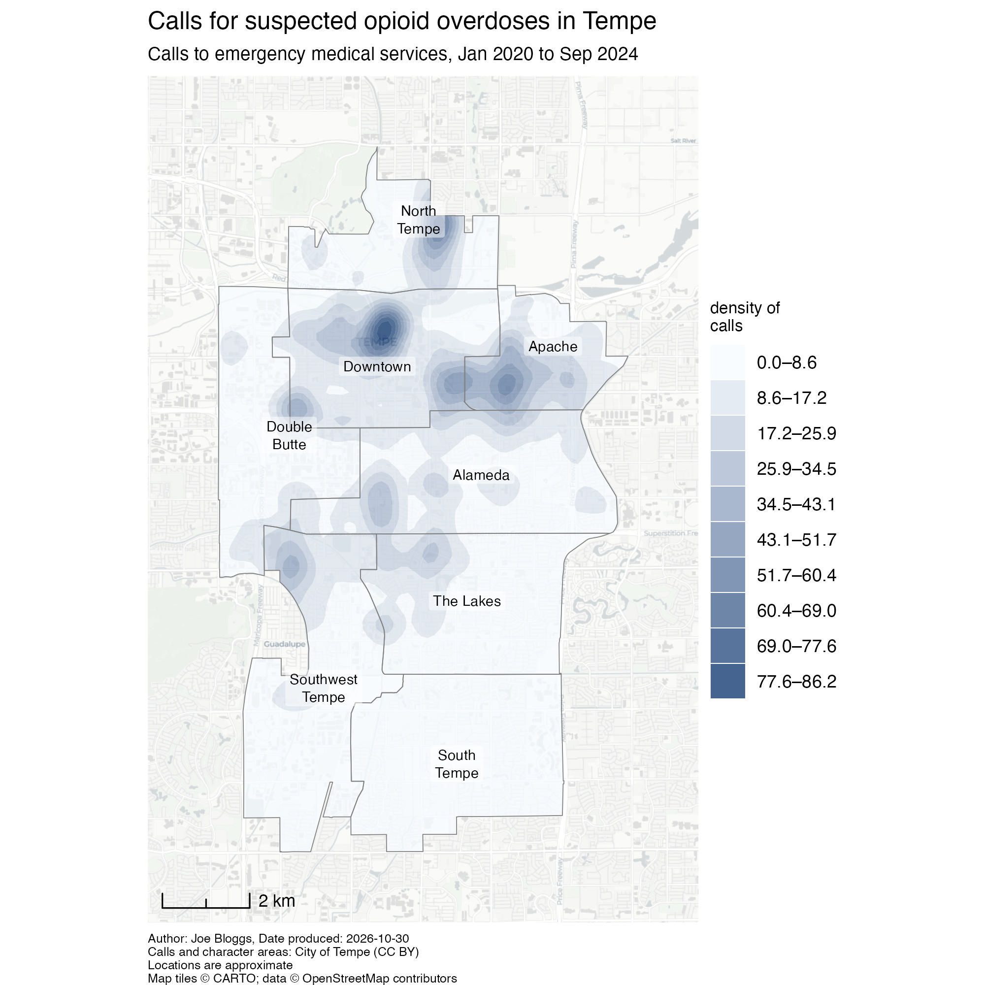
The finished map

<httr2_response>
GET https://mpjashby.github.io/crimemappingdata/tempe_opioid_calls.csv
Status: 200 OK
Content-Type: text/csv
Body: On disk '/Users/mattashby/Documents/Crime Mapping Book/exercises/data/raw/tempe_opioid_calls.csv' (125774 bytes)

<httr2_response>
GET https://mpjashby.github.io/crimemappingdata/tempe_character_areas.gml
Status: 200 OK
Content-Type: application/gml+xml
Body: On disk '/Users/mattashby/Documents/Crime Mapping Book/exercises/data/raw/tempe_character_areas.gml' (54931 bytes)

Rows: 3379 Columns: 5
── Column specification ────────────────────────────────────────────────────────
Delimiter: ","
dbl  (3): year, latitude, longitude
lgl  (1): narcan_given
date (1): incident_date

ℹ Use `spec()` to retrieve the full column specification for this data.
ℹ Specify the column types or set `show_col_types = FALSE` to quiet this message.

NoteView the complete R script

# This script produces a map of concentrations of calls to opioid overdoses in
# Tempe, Arizona, since January 2020. Run in the crime_mapping workspace.

# PREPARE ----------------------------------------------------------------------

## Load packages ----
pacman::p_load(ggspatial, here, httr2, sf, sfhotspot, tidyverse)


## Load data ----

# All data layers should be harmonised to use EPSG:6404 since this uses metres
# and covers the central part of Arizona

# Download the original data into the workspace
request("https://mpjashby.github.io/crimemappingdata/tempe_opioid_calls.csv") |>
  req_perform(path = here("data", "raw", "tempe_opioid_calls.csv"))
request(
  "https://mpjashby.github.io/crimemappingdata/tempe_character_areas.gml"
) |>
  req_perform(path = here("data", "raw", "tempe_character_areas.gml"))

# Read local calls data, keep calls since January 2020 and transform coordinates
incidents <- here("data", "raw", "tempe_opioid_calls.csv") |>
  read_csv() |>
  janitor::clean_names() |>
  filter(incident_date >= ymd("2020-01-01")) |>
  st_as_sf(coords = c("longitude", "latitude"), crs = "EPSG:4326") |>
  st_transform("EPSG:6404")

# Read the local city boundary and use the same coordinate reference system
character_areas <- here("data", "raw", "tempe_character_areas.gml") |>
  read_sf() |>
  janitor::clean_names() |>
  st_transform("EPSG:6404") |>
  # Some of the character areas have very long names which would not fit easily
  # on the map, so we abbreviate them first
  mutate(
    label = case_when(
      area_number == 1 ~ "North Tempe",
      area_number == 2 ~ "Double Butte",
      area_number == 3 ~ "Downtown",
      area_number == 7 ~ "The Lakes",
      area_number == 8 ~ "South Tempe",
      # If the area number is not specified above, use the existing area name
      TRUE ~ area_name
    )
  )


# WRANGLE ----------------------------------------------------------------------

# Estimate call density on a 200-metre grid, then clip it to the city boundary.
# Some recorded calls fall outside the boundary; a warning may be produced.
# Clipping limits the displayed density surface to the city rather than
# interpreting those approximate coordinates as exact locations.
incidents_kde <- incidents |>
  hotspot_kde(
    grid = hotspot_grid(character_areas, cell_size = 150),
    bandwidth_adjust = 0.33,
    quiet = TRUE
  ) |>
  hotspot_isoband(breaks = 10, quiet = TRUE) |>
  hotspot_clip(character_areas, quiet = TRUE)


# VISUALISE --------------------------------------------------------------------

# Create map
tempe_opioid_map <- hotspot_map(
  incidents_kde,
  basemap_type = "cartolight",
  caption = str_glue(
    "Author: Joe Bloggs, Date produced: {today()}\n",
    "Calls and character areas: City of Tempe (CC BY)\n",
    "Locations are approximate"
  )
) +
  # Add character area boundaries
  geom_sf(data = character_areas, colour = "grey50", fill = NA) +
  # Add character area labels
  geom_sf_label(
    aes(label = str_wrap(label, 10)),
    data = character_areas,
    alpha = 0.5,
    fill = "white",
    lineheight = 1,
    linewidth = 0,
    size = 2.5
  ) +
  # Add scale bar
  annotation_scale(width_hint = 1 / 5, style = "ticks", location = "bl") +
  labs(
    title = "Calls for suspected opioid overdoses in Tempe",
    subtitle = str_glue(
      "Calls to emergency medical services, ",
      "{format(min(pull(incidents, 'incident_date')), '%b %Y')} to ",
      "{format(max(pull(incidents, 'incident_date')), '%b %Y')}"
    ),
    fill = "density of\ncalls"
  ) +
  theme(
    legend.title = element_text(size = 8),
    plot.caption = element_text(hjust = 0, size = 6),
    plot.title = element_text(size = 12),
    plot.subtitle = element_text(size = 9, margin = margin(6, 0, 6, 0))
  )

# Save map
ggsave(
  here("output", "tempe_opioid_calls.jpg"),
  plot = tempe_opioid_map,
  width = 2000,
  height = 2000,
  units = "px"
)

Download the complete R script.

Step 1: Explain the script

1# This script produces a map of concentrations of calls to opioid overdoses in
# Tempe, Arizona, since January 2020. Run in the crime_mapping workspace.

1

Start by explaining that the script maps concentrations of calls for suspected opioid overdoses in Tempe since January 2020. Calls are not the same as confirmed overdoses or deaths, so it is important to describe the data accurately. See Organising code with comments.

Step 2: Load packages

# PREPARE ----------------------------------------------------------------------

## Load packages ----
2pacman::p_load(ggspatial, here, httr2, sf, sfhotspot, tidyverse)

2

pacman::p_load() loads the packages needed for this analysis, listed in alphabetical order with the tidyverse package last. ggspatial adds map elements such as scale bars; here allows us to specify where to find files in the workspace; httr2 downloads data from the internet; sf handles spatial objects; sfhotspot creates crime maps and estimates density; tidyverse provides tools for reading, wrangling and plotting data. Loading packages at the start makes it easy to check which tools the script needs. See Loading packages.

Step 3: Download the original data

## Load data ----

3# All data layers should be harmonised to use EPSG:6404 since this uses metres
# and covers the central part of Arizona

# Download the original data into the workspace
4request("https://mpjashby.github.io/crimemappingdata/tempe_opioid_calls.csv") |>
5  req_perform(path = here("data", "raw", "tempe_opioid_calls.csv"))
request(
  "https://mpjashby.github.io/crimemappingdata/tempe_character_areas.gml"
) |>
  req_perform(path = here("data", "raw", "tempe_character_areas.gml"))

3

Record the decision to use EPSG:6404 for both spatial layers. This projected CRS covers central Arizona and uses metres, which we will need when estimating density. See Choosing a projected coordinate reference system.

4

request() specifies the URL of each dataset. The first request downloads calls data; the second downloads Tempe’s character-area boundaries in GML format. These areas provide both the extent for the density layer and geographic context for the map. See Downloading and loading data.

5

req_perform() saves the requested file in data/raw. here() constructs the path relative to the workspace, so the script does not depend on a particular computer’s folder names. Keep these original files unchanged. See Keeping your files organised.

Step 4: Load and prepare the calls

# Read local calls data, keep calls since January 2020 and transform coordinates
6incidents <- here("data", "raw", "tempe_opioid_calls.csv") |>
7  read_csv() |>
8  janitor::clean_names() |>
9  filter(incident_date >= ymd("2020-01-01")) |>
10  st_as_sf(coords = c("longitude", "latitude"), crs = "EPSG:4326") |>
11  st_transform("EPSG:6404")

6

here() locates the downloaded calls file within the workspace. The pipe passes this path to read_csv(). <- stores the result of the whole pipeline as incidents.

7

read_csv() from readr reads the local calls file from the path passed through the pipe. See Loading CSV data; Stringing functions together; Naming objects.

8

janitor::clean_names() from janitor gives the columns consistent names in snake_case. See Cleaning column names.

9

filter() from dplyr keeps calls on or after 1 January 2020. ymd() from lubridate converts the text into a date that can be compared with incident_date. We do not specify an end date here; later the subtitle will identify the latest date actually present in the retained records. See Filtering rows.

10

st_as_sf() tells R to interpret the longitude and latitude columns as locations using EPSG:4326. coords lists the x and y columns, in that order. See Converting data to an SF object.

11

st_transform() changes the coordinates to EPSG:6404. Unlike the previous line, this transforms the coordinate values rather than describing the system they already use. See Transforming the coordinate reference system.

Step 5: Load the character areas and prepare their labels

12character_areas <- here("data", "raw", "tempe_character_areas.gml") |>
13  read_sf() |>
14  janitor::clean_names() |>
15  st_transform("EPSG:6404") |>
  # Some of the character areas have very long names which would not fit easily
  # on the map, so we abbreviate them first
16  mutate(
17    label = case_when(
      area_number == 1 ~ "North Tempe",
      area_number == 2 ~ "Double Butte",
      area_number == 3 ~ "Downtown",
      area_number == 7 ~ "The Lakes",
      area_number == 8 ~ "South Tempe",
      # If the area number is not specified above, use the existing area name
18      TRUE ~ area_name
    )
  )

12

here() locates the downloaded character-area file within the workspace. The pipe passes this path to read_sf(). The result of the finished pipeline is stored in a new object called character_areas.

13

read_sf() reads the downloaded GML boundaries as a spatial object, using the path passed through the pipe. The file already contains spatial information, so we do not need st_as_sf(). See Reading spatial data.

14

Clean the column names using the same convention as before.

15

Transform the character areas to EPSG:6404 as well. The areas and call locations will then use the same CRS when we calculate and clip the density layer. See Transforming the coordinate reference system.

16

mutate() adds a label column without replacing the original area names. Shorter labels are easier to fit on the map. See Transforming values.

17

case_when() chooses text according to the area number. Read each line as a condition on the left of ~ and the label to use on the right: for example, area 1 receives the label "North Tempe". You can use this supplied code without needing to write your own set of conditions.

18

TRUE ~ area_name keeps the original name for any area that did not match an earlier condition. This ensures that every area has a label.

Step 6: Calculate density, create isobands and clip the layer

# WRANGLE ----------------------------------------------------------------------

19# Estimate call density on a grid, then clip it to the character areas.
# Some recorded calls fall outside the boundary; a warning may be produced.
# Clipping limits the displayed density surface to the city rather than
# interpreting those approximate coordinates as exact locations.
20incidents_kde <- incidents |>
21  hotspot_kde(
22    grid = hotspot_grid(character_areas, cell_size = 150),
23    bandwidth_adjust = 0.33,
24    quiet = TRUE
  ) |>
25  hotspot_isoband(breaks = 10, quiet = TRUE) |>
26  hotspot_clip(character_areas, quiet = TRUE)

19

The dataset metadata tells us the recorded locations are approximate, and some fall outside the character-area boundaries. The comments explain why a warning may appear. Clipping the surface limits the displayed area; it does not correct the original locations.

20

Start with incidents and store the finished density layer as incidents_kde.

21

hotspot_kde() estimates the density of calls in each cell in a grid. See Mapping crime density.

22

hotspot_grid() defines a grid covering the character areas. cell_size = 150 makes the cells 150 metres across because the CRS of the character_areas dataset uses metres. cell_size = 150 is smaller than we might use for other cities, but Tempe is geographically a relatively small city (Tempe is a large suburb of Phoenix). See Specifying a grid for kernel density estimation.

23

bandwidth_adjust = 0.33 reduces the default smoothing bandwidth to reveal more local detail. See Fine-tuning cell size and bandwidth.

24

quiet = TRUE suppresses the progress display that is otherwise produced by hotspot_kde(). Use FALSE if you want to see progress during a long calculation.

25

hotspot_isoband() converts the gridded density estimates into polygons called isobands. breaks = 10 divides the density range into ten equal-width bands, so each polygon represents a range of density values rather than an exact value at every location. Using isobands can sometimes make patterns clearer than directly mapping the result produced by hotspot_kde(). Convert to isobands before clipping: hotspot_isoband() needs the complete grid produced by hotspot_kde(). quiet = TRUE suppresses messages telling you what settings hotspot_isoband() has automatically selected. See Converting density layers to isobands.

26

hotspot_clip() removes the parts of the density surface outside the combined character areas, while retaining the surface across the internal area boundaries. That stops the map showing density estimates outside the area selected for display. See Clipping map layers.

Step 7: Start the map and identify its sources

# VISUALISE --------------------------------------------------------------------

# Create map
27tempe_opioid_map <- hotspot_map(
28  incidents_kde,
29  basemap_type = "cartolight",
30  caption = str_glue(
    "Author: Joe Bloggs, Date produced: {today()}\n",
    "Calls and character areas: City of Tempe (CC BY)\n",
    "Locations are approximate"
  )
31) +

27

Store the finished map as tempe_opioid_map so that we can save it in a subsequent step. See Creating and storing a map.

28

hotspot_map() identifies that incidents_kde contains an isoband layer and displays its density ranges as shaded polygons over the base map, with a legend identifying the bands.

29

Choose a light cartolight base map so that streets provide context without overpowering the density layer. See Base maps.

30

str_glue() from stringr combines text with the result of processing any R code embedded in the text using braces. {today()} inserts the date the script is run. The caption credits the City of Tempe and notes that locations are approximate. Replace Joe Bloggs with your own name, or a pseudonym if you were writing this code for an assessment. See Using captions to add author and other information.

31

The + operator means the same map expression continues in the next section. These sections form one continuous stack in the complete script; they are separated here to explain each step.

Step 8: Add geographic context and map text

  # Add character area boundaries
32  geom_sf(data = character_areas, colour = "grey50", fill = NA) +
  # Add character area labels
33  geom_sf_label(
34    aes(label = str_wrap(label, 10)),
    data = character_areas,
35    alpha = 0.5,
    fill = "white",
    lineheight = 1,
    linewidth = 0,
    size = 2.5
  ) +
  # Add scale bar
36  annotation_scale(width_hint = 1 / 5, style = "ticks", location = "bl") +
37  labs(
38    title = "Calls for suspected opioid overdoses in Tempe",
39    subtitle = str_glue(
      "Calls to emergency medical services, ",
      "{format(min(pull(incidents, 'incident_date')), '%b %Y')} to ",
      "{format(max(pull(incidents, 'incident_date')), '%b %Y')}"
    ),
40    fill = "density of\ncalls"
  ) +

32

Overlay the character-area boundaries in grey. fill = NA leaves the interiors of the character area polygons unfilled so that they do not obscure the density layer. See Adding more layers; Visual hierarchy.

33

geom_sf_label() adds the character-area names so that readers can identify places where calls are concentrated. It uses the same spatial layer as the boundaries. See Adding more layers.

34

aes() specifies that the labels on the map should come from the label column in the character_areas object. str_wrap(label, 10) wraps names onto lines with a target width of 10 characters, helping them fit within the areas. It wraps between words rather than cutting words in half.

35

The labels have partly transparent white backgrounds (alpha = 0.5 and fill = "white"), compact line spacing (lineheight = 1), no border (linewidth = 0) and small text (size = 2.5). These choices help readers read the labels while keeping the density layer visually prominent.

36

Add a scale bar using ggspatial. width_hint = 1 / 5 suggests its width, style = "ticks" chooses its appearance and location = "bl" places it at the bottom left. See Scale bars.

37

labs() supplies the title, subtitle and fill-legend title. See Titles and subtitles.

38

Describe the data as calls for suspected opioid overdoses, rather than confirmed overdose deaths.

39

pull() extracts the date column, and min() and max() find the earliest and latest retained call dates. format() displays each date using an abbreviated month (%b) and a four-digit year (%Y), giving a concise range such as Jan 2020 to Sep 2024. str_glue() inserts this range into the subtitle, so it describes the downloaded records rather than assuming they extend to the present.

40

Use a short legend title that explains the colours without requiring readers to know the term KDE. \n breaks it over two lines. See Changing the legend title.

Step 9: Style the supporting text

41  theme(
42    legend.title = element_text(size = 8),
43    plot.caption = element_text(hjust = 0, size = 6),
44    plot.title = element_text(size = 12),
45    plot.subtitle = element_text(size = 9, margin = margin(6, 0, 6, 0))
  )

41

theme() from ggplot2 controls supporting elements of the map. Here it sets text sizes and spacing to give the title more prominence than the caption. See Changing the appearance of titles and captions; Visual hierarchy.

42

Set the legend title size to 8 so that it remains readable without dominating the map.

43

Left-align the caption using hjust = 0 and make it smaller than the other map text. The source information should remain readable without dominating the map. See Using captions to add author and other information.

44

Set the title size to 12 so that it is more prominent than the caption.

45

Set the subtitle size to 9 and add space above and below it. The closing brackets finish theme() and the map expression.

Step 10: Save the finished map

# Save map
46ggsave(
47  here("output", "tempe_opioid_calls.jpg"),
48  plot = tempe_opioid_map,
49  width = 2000,
  height = 2000,
50  units = "px"
)

46

ggsave() from ggplot2 writes the map to a file on your computer, using the settings on the following lines. See Saving maps.

47

Specify where the map should be saved, relative to the workspace. The file name tempe_opioid_calls.jpg also specifies the image format. See Keeping your files organised.

48

Specify the map object to save, in this case tempe_opioid_map. See Creating and storing a map.

49

Set the width and height to 2000 pixels.

50

Specify that the dimensions are measured in pixels.