5 Your second crime map – Learn Crime Mapping with R

5.1 Introduction

In Chapter 2 we produced a simple map of a particular type of crime in a neighbourhood, but we skipped over a lot of the details of how to do it. In this chapter we will make another crime map, this time focusing more on each step in the process. We will then build on this in Chapter 6 to make a better crime map.

In this chapter we will make a map of bicycle thefts in Vancouver in 2020. By the end of the chapter, you will have produced this map:

Point map of recorded bicycle thefts in Vancouver in 2020, with small semi-transparent black dots over a pale street map. The densest concentration is on the northern Downtown peninsula, with further concentrations south of False Creek and fewer points towards the southern edge. Overlapping dots make individual thefts hard to count. — Map 5.1

This isn’t a finished map, because it’s missing some of the vital elements that we’ll learn about in Chapter 6. But this map is a useful step on your journey towards being an experienced crime mapper.

In this chapter, we will learn how to:

give files informative names that work reliably in code;
describe how points, lines, polygons and rasters represent spatial data;
explain why spatial data need a coordinate reference system;
convert coordinate columns into an SF object;
filter an SF object to select particular crimes;
organise a multi-stage script using comments and blank lines; and
create and style a basic crime map using hotspot_map().

The process we will use to produce the map has four main stages:

Download

from the internet

Load

from a file into an R object

Wrangle

into the correct format for mapping

Visualise

map based on wrangled data

5.2 Naming files

Every file should have a name that helps you understand what it contains and find it again later. Good file names are easy for computers to handle, easy for people to understand and, where files have a meaningful order, sort into that order.

File names should generally follow the same conventions as object names in R: make names descriptive and use snake_case.

# Avoid
John's raw data.csv
Figure 4.jpg
DüsseldorfCrimeData.xlsx

# Prefer
john_raw_data.csv
figure_04.jpg
dusseldorf_crime_data.xlsx

Choose names that describe the contents or purpose of the file. vancouver_thefts.csv is more useful than data_file.csv.

If several scripts must run in a particular order, begin each name with a padded number:

01_wrangle_data.R
02_analyse_data.R
03_create_charts.R

The leading zero keeps the files in the correct order if the sequence grows beyond nine files.

Naming files

Which file name best follows these conventions?

Vancouver theft data 2020.csv data2.csv vancouver_thefts_2020.csv vancouver-thefts-2020 FINAL.csv

5.3 Handling spatial data

Maps are visual representations of spatial data. Spatial data is special because each row in the data is associated with some geographic feature such as a building, a street or the boundary of a neighbourhood. This adds some quirks that we have to understand to work with spatial data successfully.

Maps are made up of multiple layers of spatial data that are styled to represent features of interest and then stacked on top of one another to make the finished map. Watch this video to learn more about spatial layers and the different types of data that we can use in maps.

Video transcript: To make maps, think layers

When we make a map, we are trying to convey some information about a part of the real world. But every part of the world contains far more detail than we could ever convey easily on a map, not least because maps always show the world at a smaller scale than it really is. The infinite detail of the real world means that it can sometimes be challenging to manage all the data we want to include on a map.

In fact, to make any map we have to simplify the real world. One way to do that is to think of the world as being made up of different types of features. A feature could be something from the physical world, such as the outline of a building, the course of a street, or the location of a tree. A feature could also be a an event that happened in a particular place, such as the location of an individual crime.

There are infinite types of features that we could put on maps, but computers typically store individual features in three different ways: as points, as lines or as polygons. Points are used to represent physical features such as street lights, as well as the locations of individual events. Lines are used to represent physical features such as walls and roads, as well as behavioural features such as routes from one place to another. Polygons are used to represent features like the outline of a building or the area covered by a police force.

Most files that store spatial information can only store points, lines or polygons – not a mixture of different types. That means it’s usual for information about different types of feature to be stored in different files. For example, if we wanted to find the nearest police station to a set of crime locations, we would probably have a dataset of police station locations and a separate dataset of crime locations. Once we have all the data we need, we can build a map by adding each type of feature as a separate map layer.

Every map is made up of multiple layers of data, stacked on top of one another. For example, we might have a layer representing roads, another representing buildings, and so on. It can be easy to end up trying to show a lot of data on a map, either because the map shows a large area or because it shows a lot of detail. Eventually the amount of data becomes hard to work with. If that happens we can simplify the data by converting the points, lines or polygons on the map into a raster layer.

A raster layer is made up of a grid of cells – sometimes called pixels – with each cell having a single value associated with it. In this course we will see several examples of raster layers on maps. The first are called base maps, which show all the different physical features in an environment as a single layer. Base maps like this one can be very useful because they mean we don’t have to deal with separate layers for every type of feature we want to show on a map.

But because we can’t access each feature individually, we cannot easily choose what information is shown on a base map, or how features are represented. That means it’s important to choose a base map that shows the information we need in a clear way. Fortunately, there are lots of useful base maps available online. To summarise: Spatial data can be represent as points, lines or polygons We can build maps by stacking layers of features on top of each other We can represent features as rasters to make them easier to work with

Points, lines and polygons in spatial data are known as geometric objects or simply geometries. Spatial data is data that has a geometric object (e.g. a pair of coordinates representing a crime location) associated with each row.

5.4 Spatial data in R

Cartoon labelled sf: spatial data simplified. Monsters attach map shapes to a table with attribute columns and a geometry column. The geometry stays associated with its row while the shapes can also be drawn on a map.

There are several packages that handle raster map data from different sources. One of the most important spatial packages is the sf package, which we use to handle spatial vector data. SF stands for ‘simple features’, which is a standard for storing spatial data. SF objects are data frames that have a special column to hold the geometry (point, line or polygon) associated with each row in the data. SF objects also understand what coordinate system the geometry are described in. This means SF objects can be transformed between coordinate systems and combined together in layers on a map.

There are lots of functions in the sf package for handling spatial data. Almost all of these functions begin with the letters st_ (e.g. st_read()), which makes it easy to identify that those functions are designed to be used on SF objects.

Functions in the sf package start with the letters st_

The names of almost all functions in the sf package start with the letters st_, not the letters sf_.

5.4.1 Reading spatial data

To get started, create a new R script file to hold the permanent code for this analysis. Give the file the name chapter_05.R and save it in the same directory as the R script files we created in previous chapters. You can remind yourself how to do that by looking back to Section 2.2.

Now add the code needed to load the packages we will use for this map, including sfhotspot for the hotspot_map() function, then run that line of code. You can remind yourself how to load packages and run code in Positron by looking back to Section 2.3.1.

Code 5.1

chapter_05.R

# This script produces a map of bicycle thefts in Vancouver in 2020.

# Load packages
pacman::p_load(here, httr2, sf, sfhotspot, tidyverse)

The special features of spatial data – needing to store geometries, details of the projection used etc. – mean that spatial data is often stored in special file formats. There are lots of spatial-data formats, but fortunately almost all of them can be read by the st_read() function. This means we do not need to learn a different function for each spatial-data format.

While datasets with line or polygon geometries must almost always be stored in specific spatial-data formats, point data can also be stored in common data formats such as Excel and CSV files. The data for this chapter is provided by the Vancouver Police Department in a CSV file (gzipped to reduce the file size).

As in Section 2.3.2, we will use R to download the file into the data/raw folder before we read it. This makes the analysis more reproducible: the script records where the data came from, and the local copy remains available if the website is temporarily unavailable later.

Downloading and loading data from a CSV file

Thinking back to what we learned in Section 2.3.2, add code to chapter_05.R that downloads the dataset to data/raw/vancouver_thefts.csv.gz, then loads the local file and stores the data in an object called thefts. If you need help, you can click the ‘Solution’ button below.

We can use request() and req_perform() from the httr2 package to download the file, then use read_csv() from the readr package to load the local copy. The assignment operator <- stores the loaded data in the object thefts.

Code 5.2

chapter_05.R

# Download the raw data to a local file
request(
  "https://mpjashby.github.io/crimemappingdata/vancouver_thefts.csv.gz"
) |>
  req_perform(path = here("data", "raw", "vancouver_thefts.csv.gz"))

# Load the data into R
thefts <- read_csv(here("data", "raw", "vancouver_thefts.csv.gz"))

What does the .gz at the end of the file name mean?

CSV files can hold very large amounts of data, but at the cost of the size of the file becoming very large. We can reduce the size of a CSV file (or most other types of file) by compressing the file. You may be familiar with .zip compressed files. Gzip is another way of compressing files. Gzipped files have the file extension .gz. read_csv() can automatically decompress gzipped files, so we can treat a gzipped CSV file just the same as an uncompressed CSV file.

Viewing the first few rows of a dataset

Now that you have stored the data in the thefts object, what code is needed to view the first few rows of data? Type the code into the R Console (not the script file – see Section 2.2) and run it. Click the ‘Solution’ button to check your code.

Code 5.3

R Console

head(thefts)

5.4.2 Reading data files from your computer

The Vancouver thefts dataset consists of 21,918 rows, each representing one theft. Before we can map this data, we will need to do some minor data wrangling to get it into the format we want.

In Section 5.4.1, we downloaded the Vancouver theft data and then loaded the local file from data/raw. To load any file stored on our computer, R needs a file path that specifies where the file is stored.

You might have encountered file paths before, but you may not. A typical file path looks like this on a Mac or Linux computer:

Code 5.4

Do not run this code

/Users/john_smith/Documents/crime_mapping/data/raw/vancouver_thefts.csv

or like this on Windows:

Code 5.5

Do not run this code

C:\Users\john_smith\Documents\crime_mapping\data\raw\vancouver_thefts.csv

The important thing to note here is that computers store files such as vancouver_thefts.csv in folders (also called directories), which are themselves often stored inside larger folders, etc. A file path tells a computer where to find a particular file. The file paths in Code 5.4 and Code 5.5 can be read as telling the computer to open the Users directory, then the john_smith directory, then the Documents directory, then the crime_mapping directory (which you created in Section 1.5), and finally the file vancouver_thefts.csv.

The file paths in Code 5.4 and Code 5.5 are called absolute file paths, because they show the full location of a particular file on the computer. Absolute file paths on Windows start with X:\ (where X is a letter representing which disk drive the file is on) and with / on Mac and Linux. But there are two problems with absolute paths: they can be very long so they clutter up your code, and (more importantly) they are only correct for a specific computer. If you write an R script that includes either of those file paths, then you give that file for me to run, the code will immediately produce an error because there is no directory /Users/john_smith on my computer.

Never put absolute file paths in your code

Including absolute file paths in your code drastically increases the chances of errors when you or someone else tries to run the code on a different computer, or when you try to re-run the code later when the locations of files on your computer have changed. Always use relative file paths instead.

We can deal with that problem in a few ways. Fortunately, it’s quite simple to do as long as we always remember to:

work inside the project folder we created in Section 1.5, and
use the here() function from the here package to specify the location of files as relative paths, where ‘relative’ means relative to the project folder.

When you open the crime_mapping workspace in Positron, R knows to interpret relative file paths as being relative to the workspace folder. You can confirm the current working directory by running the function getwd() in the R Console (the ‘WD’ in getwd() means ‘working directory’).

We can construct a file path in two ways using the here() function. The first, which we’ve been using up to now, is to specify each nested folder or file as a separate argument to the here() function. For example, to open the file vancouver_thefts.csv in the raw folder that is itself inside the data folder, we would use:

Code 5.6

R Console

here("data", "raw", "vancouver_thefts.csv")

Alternatively, we can specify the file path as a single string, with each folder separated by a forward slash (/). For example:

Code 5.7

R Console

here("data/raw/vancouver_thefts.csv")

You’ll notice that when you run this code in the R Console, R prints the full file path to the file on your computer. That means you can pass the result of the here() function to any function that needs a file path, and R will know where to find the file. We have already done this in the code that loads the Vancouver thefts dataset, where we used here("data", "raw", "vancouver_thefts.csv.gz") as the file path to the local copy of the data.

Since both ways of using the here() function give the same result, you can choose to use either.

5.4.3 Cleaning column names

Cartoon of a beaver feeding awkward column names containing spaces and punctuation into a clean_names machine. Consistently formatted names emerge from the other side; the machine offers snake case and other naming styles.

Typos are one of the most frequent causes of errors in any coding language. As we learned in Section 3.2.2, column names should use snake case: lower-case letters with words separated by underscores (_). This makes code easier to read and means you do not have to remember whether a column was called crime_count, crimecount, CrimeCount or CRIMECOUNT.

At the moment, the column names in the thefts dataset are upper-case letters. Rather than having to remember this, we can easily convert them to snake case using the clean_names() function from the janitor package.

To use a function from a package, we usually first load the package using the pacman::p_load() function at the very start of a script. In this case, we probably won’t want to use any other functions from the janitor package, so instead of loading the whole package we will use this one function directly. To do this, we write the function name with the package name added to the front, separated by two colons ::.

Code 5.8

R Console

janitor::clean_names(thefts)

# A tibble: 21,918 × 10
   type         year month   day  hour minute hundred_block neighbourhood      x
   <chr>       <dbl> <dbl> <dbl> <dbl>  <dbl> <chr>         <chr>          <dbl>
 1 Other Theft  2020     1     1     0      0 11XX BURNABY… West End      4.90e5
 2 Other Theft  2020     1     1     0      0 13XX W 71ST … Marpole       4.90e5
 3 Other Theft  2020     1     1     0      1 18XX E GEORG… Grandview-Wo… 4.95e5
 4 Other Theft  2020     1     1     0      0 2X ALEXANDER… Central Busi… 4.92e5
 5 Theft from…  2020     1     1     0      0 11XX SKEENA … Hastings-Sun… 4.98e5
 6 Theft from…  2020     1     1     0     10 14XX LABURNU… Kitsilano     4.89e5
 7 Theft from…  2020     1     1     0     30 14XX W 11TH … Fairview      4.90e5
 8 Theft from…  2020     1     1     0      0 33XX OAK ST   South Cambie  4.91e5
 9 Theft from…  2020     1     1     0     30 42XX SKEENA … Renfrew-Coll… 4.98e5
10 Theft from…  2020     1     1     0      0 45XX CLANCY … Riley Park    4.92e5
# ℹ 21,908 more rows
# ℹ 1 more variable: y <dbl>

Since we always want the column names to be snake case, there’s no need for us to create a version of the data that holds the column names before we’ve cleaned them. Instead, we can use the pipe operator to add janitor::clean_names() to the code that we have already written to load the data from the CSV file. This means that the data will be loaded and the column names cleaned in one step, and we can store the result in the thefts object.

Code 5.9

chapter_05.R

# Load the data into R
1thefts <- here("data", "raw", "vancouver_thefts.csv.gz") |>
2  read_csv() |>
3  janitor::clean_names()

1: Find the location of the Vancouver thefts dataset on the specific computer you are using.
2: Load the data from the CSV file into R.
3: Clean the column names so they are in snake_case.

Add Code 5.9 to the chapter_05.R file and run that line of code. If you now run head(thefts) in the R Console, you will see that the data has stayed the same but all the column names are now in snake case. clean_names() would also have replaced any spaces with underscores, tried to separate words in the variable names and cleaned up several other potential problems. For this reason it is common to call janitor::clean_names() straight away after loading a dataset so that you can be confident that the column names will be in the format you expect.

If we wanted to use the clean_names() function again, we would have to include the package name and :: each time, so if our code was going to make repeated use of the function then it would probably be easier to load the package using the pacman::p_load() function introduced in Section 2.3.1.

5.4.4 Converting our data to an SF object

At present, the data in the thefts object is just a regular tibble. We could not use it to make a map because R does not know which columns represent the geometry, or what coordinate system the locations are recorded in. We can deal with this by converting the data to an SF object using the st_as_sf() function from the sf package.

The data provided by the Vancouver Police use the UTM zone 10N coordinate system. UTM is a system for assigning coordinates to any location on earth relative to a designated local reference point for the UTM zone covering that part of the planet. The ‘N’ at the end of the zone name 10N refers to the northern hemisphere.

Coordinate reference systems are specific to one part of the globe

In almost all cases, coordinate reference systems only work for the part of the world that they were designed for. So we should not use the UTM zone 10N coordinate system to map data outside the area for which it was designed (broadly speaking, the west coast of North America from Los Angeles to Vancouver, and the part of Canada directly north of Vancouver extending most of the way to the north pole). If we were to use the UTM zone 10N coordinate system for data from another part of the world, we would be very likely to get error messages or strange results.

A map showing Vancouver in UTM zone 10N. The neighbouring UTM zones 8N to 12N are also shown as vertical strips across western North America. — Map 5.2

We can convert the thefts tibble to an SF object using the st_as_sf() function (remember, all functions in the sf package start with st_, which can sometimes make the function names a little confusing). We specify which columns in the data represent the geometry (in this case, the x and y columns), and what coordinate system the data uses.

Coordinate systems can be specified in lots of ways (some very complicated), but the easiest is to specify the EPSG code for the relevant system. An EPSG code is a unique reference number for a particular coordinate system that R can look up in a database to get the information needed to display the data on a map. The EPSG code for the UTM zone 10N is EPSG:32610.

In Section 6.2.1, we will learn how to choose an appropriate projected CRS when one has not already been specified for us.

We only need the version of the thefts data that is a spatial dataset, so we can again add the code needed to convert the thefts tibble to an SF object to the pipeline we have already created. This means that the data will be loaded, cleaned and converted to an SF object in one step, and we can store the result in the thefts object.

Change the existing code in chapter_05.R so that it includes the st_as_sf() function in the pipeline, and run that line of code.

Code 5.10

chapter_05.R

# Load and wrangle bike theft data
1thefts <- here("data", "raw", "vancouver_thefts.csv.gz") |>
2  read_csv() |>
3  janitor::clean_names() |>
4  st_as_sf(coords = c("x", "y"), crs = "EPSG:32610")

1: Find the location of the Vancouver thefts dataset on the specific computer you are using.
2: Load the data from the CSV file into R.
3: Clean the column names so they are in snake_case.
4: Convert the tibble to an SF object, specifying which columns represent the geometry and what coordinate system the data uses.

Rows: 21918 Columns: 10
── Column specification ────────────────────────────────────────────────────────
Delimiter: ","
chr (3): TYPE, HUNDRED_BLOCK, NEIGHBOURHOOD
dbl (7): YEAR, MONTH, DAY, HOUR, MINUTE, X, Y

ℹ Use `spec()` to retrieve the full column specification for this data.
ℹ Specify the column types or set `show_col_types = FALSE` to quiet this message.

If you look at the contents of the thefts object by running head(thefts) in the R Console, you’ll see that there is a new column called geometry. This column contains the coordinates of each bike theft. But crucially, it stores those coordinates in a format that R recognises represent specific locations on the surface of the earth, which means the coordinates can be used to make maps.

Only convert non-spatial data with st_as_sf()

It is important to remember that we should only use st_as_sf() to convert a non-spatial dataset (such as a tibble) into a spatial dataset (an SF object). If we use st_as_sf() on an object that is already an SF object, this can have unexpected results and lead to errors in your code.

The easy way to think about this is that if you have loaded a dataset with read_sf() or st_read() then you have already created an SF object, so you don’t need st_as_sf(). If you have loaded a dataset with any other function that reads data (such as read_csv() or read_excel()) then you will need to use st_as_sf() if you want to plot the data on a map. Most importantly, do not use st_as_sf() if you loaded a dataset with read_sf() or st_read().

5.4.5 Finding bike thefts in our data

Choosing only some rows in a dataset

If you look through the contents of the thefts object by running head(thefts) in the R Console, you will see that not all of the rows relate to bicycle thefts. The type column shows that the dataset also includes thefts from vehicles, for example. To choose only those rows containing bicycle thefts, which function from the dplyr package would we use? If you need help, you can think back to Chapter 3 or have a look at the Data transformation with dplyr cheat sheet.

Which function from the dplyr package should we use to remove all the rows from our dataset except those for bicycle thefts?

select() filter() mutate() summarise()

Add code to the chapter_05.R file to create a new object called bike_thefts that contains only the rows in the thefts object that relate to bicycle theft. If you get stuck, you can hit the ‘Hint’ button below to get help, but try to find the answer on your own first! Once you’ve finished the code, click the ‘Solution’ button to check your code.

Use the filter() function to choose particular rows in a dataset. The syntax for filter() is filter(dataset, column_name == "value"). Replace dataset with the name of the SF object we created above, column_name with the name of the column containing the offence type and value with the offence type for bicycle theft.

The correct code to store only bicycle thefts in a new object is:

Code 5.11

chapter_05.R

bike_thefts <- filter(thefts, type == "Theft of Bicycle")

Our data is now ready for us to make our crime map!

5.5 Organising code with comments

The script in this chapter now performs several tasks in sequence: it loads packages, downloads and reads data, cleans column names, converts the data to a spatial format and selects bicycle thefts. Comments and blank lines make those stages easier to recognise.

Add a comment at the top of a script to explain its overall purpose. Comments begin with # followed by a space and should normally use standard capitalisation and punctuation.

# This script produces a map of bicycle thefts in Vancouver in 2020.

Use a short comment above each distinct task to explain why that block exists. You don’t necessarily need to annotate every single line of code if what that line does it obvious, but if you prefer to add a comment above every line to help yourself understand what the code does, that’s fine.

# Load packages
pacman::p_load(here, httr2, sf, sfhotspot, tidyverse)

# Load and prepare the theft data
thefts <- here("data", "raw", "vancouver_thefts.csv.gz") |>
  read_csv() |>
  janitor::clean_names() |>
  st_as_sf(coords = c("x", "y"), crs = "EPSG:32610")

Leave a blank line between separate tasks, but do not add blank lines within a pipeline. The result is code that is visually grouped in the same way as the analytical process.

For a longer script, a comment ending with at least four hyphens creates a section heading:

# Load data ----

# Wrangle data ----

# Produce map ----

Positron recognises these headings, allows the sections to be folded and treats them as boundaries between code cells. They make it easier to move through and run a long script one stage at a time.

Comments

Which is the best comment to place above code that loads a dataset?

#Load data # Load data # load data # READ_CSV

5.6 Producing maps in R

Now that we have our data, we can use it to create a map of bicycle theft in Vancouver. Before we start, let’s take another look at our dataset so that we know which columns contain which data.

Code 5.12

R Console

head(bike_thefts)

Simple feature collection with 6 features and 8 fields
Geometry type: POINT
Dimension:     XY
Bounding box:  xmin: 488371.3 ymin: 5452696 xmax: 494295.1 ymax: 5458232
Projected CRS: WGS 84 / UTM zone 10N
# A tibble: 6 × 9
  type              year month   day  hour minute hundred_block    neighbourhood
  <chr>            <dbl> <dbl> <dbl> <dbl>  <dbl> <chr>            <chr>        
1 Theft of Bicycle  2020     1     1     0      0 12XX VENABLES ST Strathcona   
2 Theft of Bicycle  2020     1     1     0      0 20XX MAPLE ST    Kitsilano    
3 Theft of Bicycle  2020     1     1    13      0 7XX PACIFIC BLVD Central Busi…
4 Theft of Bicycle  2020     1     1    20      0 53XX VINE ST     Arbutus Ridge
5 Theft of Bicycle  2020     1     3    11     55 65XX ANGUS DR    Kerrisdale   
6 Theft of Bicycle  2020     1     3    14      0 4XX E 10TH AVE   Mount Pleasa…
# ℹ 1 more variable: geometry <POINT [m]>

Since we have converted the data to an SF object, it is easy to create a basic map using the hotspot_map() function that we were introduced to in Chapter 2. In the background, this function does several things to put together a map so that we don’t have to do that ourselves.

hotspot_map() only works with SF objects

hotspot_map() only works on SF objects, which is why we needed to convert the original tibble of data to an SF object using st_as_sf(). If you try to use hotspot_map() on a dataset that is not stored as an SF object, R will produce an error.

The most-basic crime map that we can make simply plots the locations of crimes, with no context other than a base map (we’ll learn more about base maps in Section 7.7). Run this code in the R Console to produce a basic map:

Code 5.13

R Console

hotspot_map(bike_thefts)

Point map of recorded bicycle thefts in Vancouver in 2020 over a coloured street map. Large black circles overlap into a nearly solid patch on the Downtown peninsula and obscure streets in other concentrations, making individual incidents difficult to distinguish. — Map 5.3

Map 5.3 shows the bike-theft data, but it is obviously not a very useful map. Fortunately, we can use some features of the hotspot_map() function to improve it.

Avoid dot maps

Unless we want to produce a map of only a very small number of crimes (like the Atlanta downtown homicides map we produced in Chapter 2), it is unlikely that a point map will be very useful. A dot map like this almost never makes a good crime map because if there are more than a few crimes it becomes hard to see patterns in the data.

If you find yourself making a map with each crime represented by a separate point, you should probably stop and ask yourself if that is really the best way to achieve your goal – it will almost always be better to map the data in another way.

We are only creating a dot map in this chapter because it is a simple way to introduce the basic principles of making maps in R. In Chapter 6 we will learn how to make more useful maps that show patterns of crime more effectively.

5.6.1 Controlling aesthetics

We can change the appearance of the points by specifying various arguments to the hotspot_map() function. These arguments are called aesthetics, because they control the aesthetic appearance of the geometric objects (points, lines etc.) that are added to the map. There are lots of aesthetics, but some of the most common are:

colour controls the colour of points and lines (for polygons, it controls the colour of the border around the polygon edge) – you can also use the spelling color for this argument and get an identical result,
fill controls the colour used to fill polygons or points that use a shape capable of having different colours in the centre and around the edge (fill has no meaning for lines),
shape controls the shape (circle, triangle, square etc.) of points (it has no meaning for lines or polygons),
size controls the size of points and text,
linewidth controls the width of lines, including the borders around the edges of polygons, and
alpha controls the transparency of a layer (alpha = 1 equals fully opaque, alpha = 0 means fully transparent).

colour and fill can be specified using any one of 657 R colour names or using a hexadecimal (‘hex’) colour code. Values of size don’t relate to any common unit of size (e.g. millimetres or points), so it’s easiest to set the size of points and text by trial and error.

There are 25 built-in shapes for points in R (shape 16 is the default):

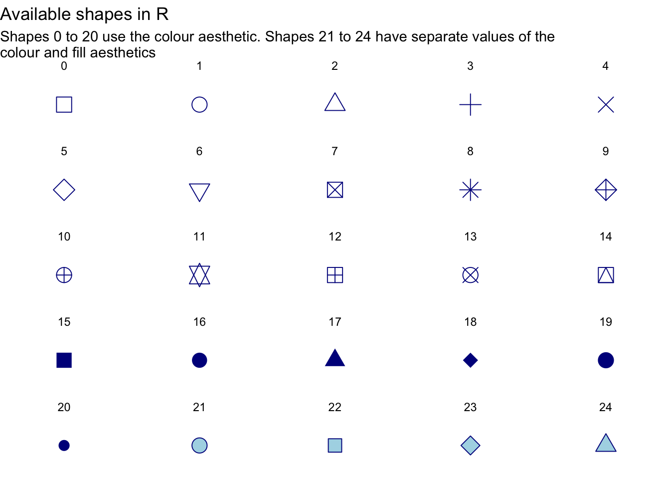
Grid of R point symbols numbered zero to twenty-four, arranged in rows of five. It includes outlined and filled squares, circles, triangles and diamonds, plus crosses and combined symbols. Symbols twenty-one to twenty-four have separately controllable outlines and fills. A symbol key follows.

Image description: R point symbols

The grid runs left to right in rows of five. The number supplied to shape selects the following symbol:

Number	Symbol
0	Outlined square
1	Outlined circle
2	Upward-pointing outlined triangle
3	Plus
4	Diagonal cross
5	Outlined diamond
6	Downward-pointing outlined triangle
7	Square with diagonal cross
8	Plus with diagonal cross
9	Diamond with plus
10	Circle with plus
11	Overlapping upward- and downward-pointing triangles
12	Square with plus
13	Circle with diagonal cross
14	Square with downward-pointing triangle
15	Filled square
16	Filled circle
17	Filled upward-pointing triangle
18	Filled diamond
19	Filled circle
20	Small filled circle
21	Circle with separate outline and fill
22	Square with separate outline and fill
23	Diamond with separate outline and fill
24	Upward-pointing triangle with separate outline and fill

Symbols 0 to 20 use colour; symbols 21 to 24 in this grid allow separate colour and fill settings.

We use aesthetics such as colour, fill, etc. to change the appearance of layers on a map by adding the aesthetic as an argument to the hotspot_map() function. For example, we could change the points on our map to be red squares rather than the default black circles using this code:

Code 5.14

R Console

# Create a basic crime map
hotspot_map(bike_thefts, shape = 15, colour = "red")

Point map of recorded bicycle thefts in Vancouver in 2020, with red squares replacing the default black circles over the same street map. Dense overlapping squares obscure individual incidents, particularly on the Downtown peninsula; changing shape and colour alone has not resolved the overlap. — Map 5.4

As we have said, this basic map is not very useful. We can see that there seems to be a cluster of bike thefts towards the top (north) of the map, but it is difficult to see how important this cluster is because so many of the points overlap. Overlapping points are a particular problem in maps, because if there are multiple crimes at the same location then the points representing those crimes will be exactly on top of one another and it will be impossible to see whether there is one crime at a particular location or 100.

One way to deal with this problem is to make the points semi-transparent so that overlapping points appear darker. This often works better if we also make the points slightly smaller at the same time. We can use the alpha and size aesthetics to make the points smaller (relative to the default for points of size = 1) and semi-transparent.

Add this code to your script file:

Code 5.15

chapter_05.R

# Create a basic crime map
hotspot_map(bike_thefts, basemap_type = "cartolight", size = 0.7, alpha = 0.1)

Point map of recorded bicycle thefts in Vancouver in 2020, with small semi-transparent black dots over a pale street map. Darker overlapping areas reveal concentrations on the Downtown peninsula and south of False Creek, while scattered dots extend across the rest of the city. — Map 5.5

Making the points semi-transparent goes some way to making it easier to see where bike theft is most common in Vancouver, but the pattern is not clear and it is not possible to tell which darker points represent a handful of crimes at the same location and which represent hundreds of crimes at the same location.

To make our map truly useful, we need to use a different technique. In Chapter 6 we will learn how to identify crime patterns by mapping the density of crime. We will also learn more about aesthetics in Section 6.6.

Producing maps in R

What is the effect of setting alpha to a value below 1?

It changes the coordinate reference system It removes points outside the map It makes points semi-transparent It changes the point shape

Why should we be cautious about using a dot map for a large crime dataset?

A dot map always hides the location of individual crimes Many overlapping points can make the number and pattern of crimes difficult to interpret geom_sf() cannot display more than 100 points Dot maps can only display polygon data

Save chapter_05.R by pressing . Then start a new R session by clicking the Restart R (⟳) button in Positron’s Console panel. This creates a blank canvas for Chapter 6.

5.7 In summary

In this chapter we have learned more about some of the specific steps in the process of creating a basic crime map. Concepts such as coordinate reference systems and EPSG codes can be hard to understand at first, and we will practise applying them as we make more maps throughout this book.

We have practised how to:

give data and script files informative names;
distinguish between point, line, polygon and raster spatial data;
explain why spatial data need an appropriate coordinate reference system;
download a raw-data file without overwriting an existing copy;
use project-relative paths to load local data;
convert coordinate columns into an SF object;
use a pipeline to prepare spatial data;
organise a script using comments, blank lines and section headings; and
draw and style spatial points using hotspot_map().

At the moment, your script file should look like this.

Code 5.16

chapter_05.R

# This script produces a map of bicycle thefts in Vancouver in 2020.

# Load packages
pacman::p_load(here, httr2, sf, sfhotspot, tidyverse)

# Download the raw data to a local file
request(
  "https://mpjashby.github.io/crimemappingdata/vancouver_thefts.csv.gz"
) |>
  req_perform(path = here("data", "raw", "vancouver_thefts.csv.gz"))

# Load and wrangle bike theft data
thefts <- here("data", "raw", "vancouver_thefts.csv.gz") |>
  read_csv() |>
  janitor::clean_names() |>
  st_as_sf(coords = c("x", "y"), crs = "EPSG:32610")

bike_thefts <- filter(thefts, type == "Theft of Bicycle")

# Create a basic crime map
hotspot_map(bike_thefts, basemap_type = "cartolight", size = 0.7, alpha = 0.1)

The limitations of this map

At the moment, it isn’t very easy to see patterns on this map, since so many of the points overlap. In Chapter 6, we will learn how to make this map much better by converting it into a density map.

Remember: whenever you find yourself creating a dot map, ask yourself if a density map would be more useful.

You can find out more about some of the things we have covered in this chapter using these resources:

Understand more about the history of trying to develop accurate map projections in this short video: Why all world maps are wrong.
Learn more about making maps using simple features in Chapter 1 of Spatial Data Science by Edzer Pebesma and Roger Bivand.

Revision questions

Answer these questions to check you have understood the main points covered in this chapter. Write between 50 and 100 words to answer each question.

What is spatial data, and how does it differ from other types of data? Provide examples of spatial features commonly used in crime mapping.
Explain the role of coordinate systems in mapping. Why is it important to use the correct coordinate system for a specific dataset?
Discuss the challenges of using file paths in R scripts and how relative file paths improve code portability.
Why is it helpful to use the pipe operator (|> in R) when working with multiple functions? Provide an example from the chapter.
What information does st_as_sf() need to convert a non-spatial dataset into an SF object, and why is each part needed?

Artwork by Allison Horst

5.1 Introduction

5.2 Naming files

5.3 Handling spatial data

5.3.1 Representing places on the earth

5.4 Spatial data in R

5.4.1 Reading spatial data

5.4.2 Reading data files from your computer

5.4.3 Cleaning column names

5.4.4 Converting our data to an SF object

5.4.5 Finding bike thefts in our data

5.5 Organising code with comments

5.6 Producing maps in R

5.6.1 Controlling aesthetics

5.7 In summary