16  Mapping crime series

In this chapter we will learn to map crime series, a sequence of crimes committed by the same individual or group. Using a historical case study, we will learn how to visualise crime series by mapping linked cases.

TipBefore you start

1. Open Positron or – if you already have Positron open – start a new R session by clicking the Restart R (⟳) button in the Console panel. This makes sure no code you ran previously will interfere with the work you do in this chapter.
2. Make sure you are working in the crime mapping project workspace you created in Section 1.5. In the top-right corner of the Positron window, you should see a folder icon and the words crime_mapping. If not, click the File menu, then Open Folder … and choose the crime_mapping folder.

16.1 Introduction

Up until now we’ve mapped each crime in a dataset as a separate event. This is very common in crime mapping, and is useful for many purposes. But a large proportion of crimes are committed by a relatively small proportion of all the people who commit crime. These persistent or repeat offenders commit crimes frequently, maybe several times a day in the case of some people. One type of repeat offending is the crime series, in which an offender or group of offenders commits the same or related crimes in different places over time. If we are trying to understand a crime series, it is important to map the sequence of events, rather than treating each crime as a separate event. In this chapter we will learn how to map crime series.

16.1.1 Case linkage

One of the difficulties in studying serial offending is in identifying which offences are committed by the same offender. Case linkage is the process of identifying crime series by looking for similarities in the method used by an offender (e.g. entering a house by breaking a lock on a side door out of sight from the street) or by evidence left at the scene (such as fingerprints or DNA). Case linkage is typically an imperfect process – investigators might believe that two offences were committed by the same person, but in most cases they are unlikely to know for sure unless the offender has been caught (and sometimes not even then).

Watch this video to learn a bit more about crime linkage.

TranscriptVideo transcript: What Is Crime Linkage?

This transcript starts at 0:13, matching the starting point of the video above.

Crime linkage is the practice of identifying which different offenses were committed by the same offender. For example, if you have a whole lot of unsolved burglaries, you want to find out which offenses are attributable to the same person. That is because you might have some information about the perpetrator from one crime, for example, a shoe print that points to a male with a certain shoe size and weight. See if you could identify which other offenses you think are linked to that same person.

Perhaps some of those have other information about the burglar, such as a witness seeing that he has a tattoo on one hand. And in this way, you can put together more and more pieces of the puzzle. You now have good reasons to believe that the offender who is responsible for this particular series is of a certain gender, weight, has a certain shoe size, which might point to his approximate height, and he has a tattoo on one hand.

If you allocate one of those pieces to the wrong puzzle, i.e., to the wrong series of offenses, you unnecessarily hinder the investigation. So, it’s important to link the right offenses to the right person. Crimes can be linked through the perpetrator’s MO, or modus operandi, which is how he carries out his crimes. This can refer to the kind of targets he selects and what he does to those targets. For example, Jack the Ripper’s MO was to attack prostitutes in London’s Whitechapel area in the East End during darkness and to cut their insides.

If another prostitute was poisoned to death in a different part of London during the day, that would not be consistent with Jack’s MO, and we might therefore regard that as being the crime of another person. People are creatures of habit, and if we find a way of doing something that works, we tend to stick with that way of doing it as we have learned that it is effective. A skilled burglar who knows how to pick locks is unlikely to kick the door down.

He is much more likely to continue picking locks as that gets him through doors quietly. So we’re looking for commonalities in decisions taken by the offender, how and whom he targets and how and whom he attacks for example. We also need to take into account progression. A prolific offender might gain at least experience but perhaps also additional skills during the commission of each crime. When he makes a mistake on one occasion for example that nearly got him caught, he might take care to avoid that or prepare for it next time round.

As we’re looking for both consistency across time but also progression, it is important to identify in which order the offenses took place. Criminals also tend to become increasingly confident as they continue in their offending without getting caught. So they might be willing to take more and more risks. Of course, the most reliable factor to use when linking crime is forensics so that when you find an offender’s DNA at every burgled property, you can safely assume he has been there.

MO is another way of linking crimes but it is not as reliable as geography which I will introduce next. Thank you for watching. I hope you found this content useful. You can get access to each episode’s transcript with key learning points, timestamps and references if you get yourself onto my mailing list. Just go to the main website on police science doctor.com and on the bottom of each page you will find a sign up form for notifications of new content.

Just enter your first name, your preferred email address and the type of organization you work for. You will not get any spam. This is just for me to let you know about new content and for you to get access to all the transcripts.

QuizCase linkage

What is the primary goal of case linkage?

To determine the time a crime was committed To identify which offences were committed by the same offender To analyse the psychological state of the offender To predict where future crimes will occur

Which of the following is an example of an offender’s modus operandi (MO)?

The specific methods the offender uses to carry out their crimes The DNA evidence left behind at the crime scene The legal defence strategy used by the offender in court The geographical location where the crimes occur

According to the video, what is the most reliable factor to use when linking crimes?

The offender’s modus operandi The geographical locations of the crimes Forensic evidence, such as DNA The type of victim the offender targets

16.1.2 The case used in this chapter

Due to the inherent uncertainty of case linkage, there is little publicly available data on the locations of serial crimes. The available data tend to focus on serial murders, since murder is the crime that is most likely to be solved (in most developed countries, a very high proportion of murders are solved). To minimise the likelihood of anyone reading this book having been directly affected by – or knowing anyone affected by – the cases we use in this chapter, we will use a historical example.

The Hungerford massacre occurred in southern England in August 1987, when a marauding attacker (also known as a spree offender) killed 16 people and shot many others in the space of about 90 minutes. We will use a dataset called hungerford_shootings that contains the names of each victim and the approximate location at which they were shot (recorded as eastings and northings in the British National Grid). This data is taken from the official report into the massacre. Each row represents a shooting location, so some rows contain more than one victim. The order column shows the sequence of locations rather than numbering individual victims. These are the first few rows of the dataset (the dagger symbol † shows that the victim was killed, rather than non-fatally injured):

victims	order	easting	northing
Susan GODFREY†	1	423168	167694
Kakaub DEAN	2	429455	167904
Roland MASON†, Sheila MASON†, Marjorie JACKSON, Lisa MILDENHALL	3	433849	168176
Kenneth CLEMENTS†	4	434044	168133
Roger BRERETON†, Linda CHAPMAN, Alison CHAPMAN	5	433897	168165

In this chapter we will learn how to create this composite map of the locations of the shootings in this crime series.

Map 16.1

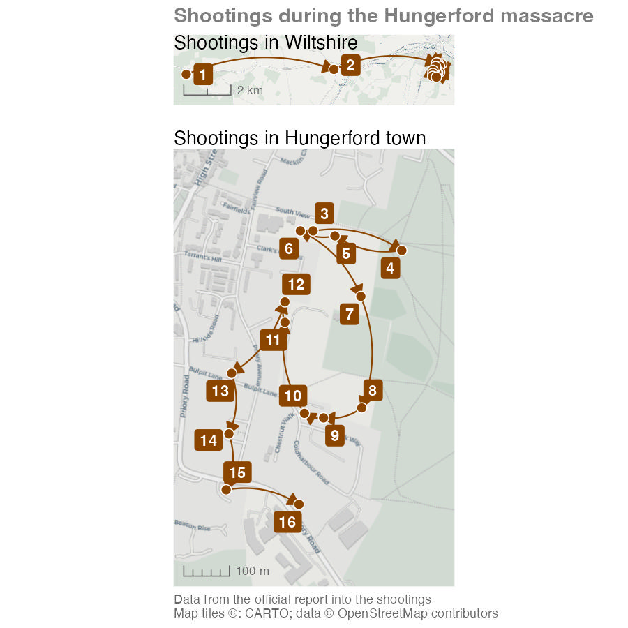
NoteMap description: the Hungerford shooting sequence

The two maps use different scales. In the upper map, location 1 is furthest west in Wiltshire. An arrow runs east to location 2, then onwards to the tightly packed locations in Hungerford. The scale bar represents 2 kilometres.

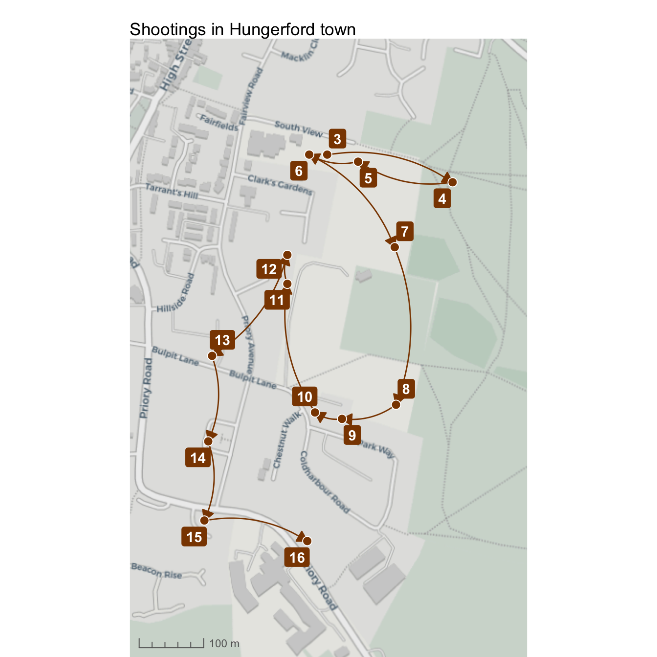
The lower map enlarges locations 3 to 16 in the town, with a 300-metre scale bar. Starting in the north, arrows link 3 to 4 to the east, then turn west through 5 and 6. The sequence runs south through 7, 8 and 9, then north-west through 10, 11 and 12. It then moves south along the western side through 13, 14 and 15, east to 16 and back north towards the earlier locations. The numbers indicate the order of shooting locations, rather than the number of victims. Arrows connect recorded locations; they do not identify every street travelled along.

In this chapter, we will learn how to:

• prepare an ordered sequence of events for mapping using arrange() and lag();
• connect event locations using curved lines and directional arrows;
• expand the area displayed on a map;
• add labels that are automatically offset from the points they relate to;
• create overview and detailed maps of the same events; and
• combine multiple maps into one output using the patchwork package.

Create a new R script file in Positron and save it as chapter_16.R in the R folder of the workspace you created in Section 1.5. Add this code to download the original data into data/raw, load the local copy and prepare to make the map. Run the code by pressing .

Code 16.1

chapter_16.R

# This script creates a combination of maps showing the sequence of shootings
# during the Hungerford massacre in 1987

# Load data --------------------------------------------------------------------

# Load packages
pacman::p_load(ggrepel, ggspatial, here, httr2, patchwork, tidyverse)

# Download the original shootings data
request(
  "https://mpjashby.github.io/crimemappingdata/hungerford_shootings.csv"
) |>
  req_perform(path = here("data", "raw", "hungerford_shootings.csv"))

# Load the local copy of the shootings data
hungerford_shootings <- here("data", "raw", "hungerford_shootings.csv") |>
  read_csv() |>
  arrange(order)

<httr2_response>
GET https://mpjashby.github.io/crimemappingdata/hungerford_shootings.csv
Status: 200 OK
Content-Type: text/csv
Body: On disk '/Users/mattashby/Documents/Crime Mapping Book/data/raw/hungerford_shootings.csv' (798 bytes)

Rows: 16 Columns: 4
── Column specification ────────────────────────────────────────────────────────
Delimiter: ","
chr (1): victims
dbl (3): order, easting, northing

ℹ Use `spec()` to retrieve the full column specification for this data.
ℹ Specify the column types or set `show_col_types = FALSE` to quiet this message.

You might notice this code loads some packages we haven’t worked with before. We’ll introduce these packages in this chapter.

16.2 Mapping linked cases

Mapping crime series can be useful for several reasons. For example, a map of a crime series might help the jurors in a criminal trial to better understand the sequence of events that the suspect is accused of. This can be especially helpful if the sequence is complicated or especially long.

At the moment, the hungerford_shootings dataset contains the point location of each event and the order in which they occurred. To show a sequence of events on a map, we need to link each event with those that happened immediately before and after it.

victims	order	easting	northing
Susan GODFREY†	1	423168	167694
Kakaub DEAN	2	429455	167904
Roland MASON†, Sheila MASON†, Marjorie JACKSON, Lisa MILDENHALL	3	433849	168176
Kenneth CLEMENTS†	4	434044	168133
Roger BRERETON†, Linda CHAPMAN, Alison CHAPMAN	5	433897	168165

One way to do that is to draw lines on the map connecting each incident in turn. To do this, we will create a dataset where each row contains two pairs of coordinates: one representing the location of a particular shooting and the other representing the location of the previous shooting. To do that, we will:

1. Take the hungerford_shootings dataset and rename the existing columns holding the coordinates so that it is clear those coordinates are for the end of each line between points. To do this we will use the rename() function from the dplyr package.
2. Sort the rows using the order column. This is essential because lag() uses the current row order when it retrieves the previous value.
3. Add two new columns to each row that show the coordinates of the row in the dataset immediately above the current row (i.e. the row that represents the location before the current location). We will do this with the lag() function, also from dplyr.
4. Use these two pairs of coordinates to plot lines on a map.

Code 16.2

chapter_16.R

# Prepare data -----------------------------------------------------------------

# Create dataset of lines joining shootings in sequence
hungerford_lines <- hungerford_shootings |>
  # Arrange the rows in order of the sequence of shootings
  arrange(order) |>
  # Make it clear the coordinates refer to the coordinates we want to use for
  # the *end* of each line, to distinguish them from the second set of
  # coordinates we'll create next
  rename(x_end = easting, y_end = northing) |>
  # Copy the coordinates from the row above each row to create a second set of
  # coordinates for the *start* of each line
  mutate(x_start = lag(x_end), y_start = lag(y_end)) |>
  # Remove the first row, which now contains missing values for `y_start` and
  # `x_start`, and which we don't need
  drop_na(x_start, y_start)

Code 16.3

R Console

head(hungerford_lines)

# A tibble: 6 × 6
  victims                                    order  x_end  y_end x_start y_start
  <chr>                                      <dbl>  <dbl>  <dbl>   <dbl>   <dbl>
1 "Kakaub DEAN"                                  2 429455 167904  423168  167694
2 "Roland MASON†\nSheila MASON†\nMarjorie J…     3 433849 168176  429455  167904
3 "Kenneth CLEMENTS†"                            4 434044 168133  433849  168176
4 "Roger BRERETON†\nLinda CHAPMAN\nAlison C…     5 433897 168165  434044  168133
5 "Abdur KHAN†\nAlan LEPETIT\nHazel HASLETT…     6 433821 168176  433897  168165
6 "Betty TOLLADAY"                               7 433954 168032  433821  168176

TipWhy does this code include drop_na()?

You might notice that the values in the first row of the x_start and y_start columns in the hungerford_lines object are NA values. This is because these columns have been created using the lag() function, which gets the value from the same column in the row immediately above. The first row doesn’t have a row immediately above it, so lag() returns NA. Since the first row does not represent a link between shootings in any case, we can remove it with drop_na().

This method for creating lines between points is one of several ways we could achieve the same result. For example, we could create lines connecting the points and store them as SF objects. However, the code to do that is more complicated and would give us slightly less control over the appearance of the lines.

Using this method means the points and lines we want to put on our map are not SF objects, so we cannot use geom_sf() to add them to the map. Instead, we will add the points representing shooting locations to the map using geom_point() and add the lines between points using geom_segment(), both from the ggplot2 package. Since hotspot_map() only works for SF objects, we cannot use hotspot_map() in this case, either. That means we have to do some things manually that would normally be done for us automatically. The extra code in Code 16.4 is explained in the accompanying notes.

Run this code in the R Console.

Code 16.4

R Console

# Plot a basic map
ggplot() +
  # Add base map
  annotation_map_tile(type = "cartolight", zoomin = 0, progress = "none") +
  # Add lines between points
  geom_segment(
    aes(x = x_start, y = y_start, xend = x_end, yend = y_end),
    data = hungerford_lines
  ) +
  # Add points
  geom_point(aes(x = easting, y = northing), data = hungerford_shootings) +
  # Since our layers are not an SF object, tell `ggplot()` what coordinate
  # system to use
  coord_sf(crs = "EPSG:27700") +
  # Add base map attribution statement
  labs(caption = "Map tiles ©: CARTO; data © OpenStreetMap contributors") +
  theme_void()

Map 16.2

1. When we make a map using hotspot_map(), in the background that function uses the annotation_map_tile() function (from the ggspatial package) to add a base map to the map. Since we’re not using hotspot_map(), we have to do this ourselves.
2. Since we aren’t using SF objects, we need to tell ggplot() how to translate the coordinates in our data to locations on the map. We do this with the coord_sf() function.
3. hotspot_map() automatically adds a caption to the map to acknowledge the source of the base map tiles used on a particular map (see Section 7.7), so here we have to do this ourselves.
4. We use theme_void() to remove information that is often useful for a chart but not for a map, such as labels along the x- and y-axes showing coordinates.

This map is not particularly useful – we will improve it in Section 16.2.1 and Section 16.2.2.

If you look at this code, you’ll see that we’ve included the function coord_sf() in our ggplot() stack. In all the previous maps that we have made, we have used geom_sf() to plot geographic data on our maps. geom_sf() understands how to translate coordinates specified using different coordinate systems to locations on the surface of each map. Other functions in the geom_*() family of functions do not know how to do this automatically, so we must specify the coordinate system by adding the coord_sf() function to the stack. We only need to use one argument to coord_sf(): the crs argument to specify the coordinate system that our data uses. In this case, we know that the coordinates in the hungerford_shootings and hungerford_lines objects are specified using the British National Grid, which has the EPSG code EPSG:27700.

Map 16.2 shows the sequence of events, but there are at least four ways that we can make it better.

1. It would be useful to be able to see a larger area around the shooting locations, to see more of the town surrounding the area in which the crimes occurred.
2. We don’t know which order to move through the sequence of lines. We can deal with this by adding arrows to show the direction in which the sequence progressed.
3. The straight lines make it look like the offender travelled across fields between locations, which is probably not true. Since we do not have data on what routes the offender took, we can replace the straight lines with curves to indicate that the exact route is unknown.
4. Because the first two shootings occurred outside the town, the map has to cover a large area and this makes it harder to see the sequence of events in the town itself.

16.2.1 Extending the map area

By default, ggplot() works out the limits of the area shown on the map based on the area covered by the data we add to each stack with functions from the geom_*() family of functions. Usually this works well, but in this case the distribution of the shootings means that the map shows only a small slice of the town of Hungerford and the surrounding area. It would be useful for readers to be able to see a larger area, to be able to better identify where the shootings occurred.

We can increase the size of the area shown on the plot in two ways. We could use the fixed_plot_aspect() function from the ggspatial package to control the aspect ratio of the plot (i.e. how tall it is relative to how wide it is). With some trial and error, we could use this to determine the best aspect ratio for showing the data on this map. However, this only allows us to control the overall size of the plot, not the amount of space around the data in each direction.

For more-specific control over what area is shown, we can use the scale_x_continuous() and scale_y_continuous() functions from the ggplot2 package. We used the scale_fill_distiller() function in Section 7.6 to control how columns in the data are represented as colours on the map. The scale_x_continuous() and scale_y_continuous() functions are similar, in that they control the horizontal (X) and vertical (Y) axes on the map. We don’t need to use most of the capabilities of these because ggplot() sets reasonable default values. The only argument we need to set is the expand argument, which controls how far the map should extend around the area covered by the data.

The easiest way to set the correct values for the expand argument is to use the expansion() helper function. We can use this to specify how much extra area around the data we want to include on the map. For example, expansion(2) means that the axis of the map should cover the area covered by the data and twice that distance either side of the data.

Run this code in the R Console.

Code 16.5

R Console

# Plot a basic map
ggplot() +
  # Add base map
  annotation_map_tile(type = "cartolight", zoomin = 0, progress = "none") +
  # Add lines between points
  geom_segment(
    aes(x = x_start, y = y_start, xend = x_end, yend = y_end),
    data = hungerford_lines
  ) +
  # Add points
  geom_point(aes(x = easting, y = northing), data = hungerford_shootings) +
  # Expand the map to show a larger area above/below the data
  scale_y_continuous(expand = expansion(2)) +
  # Specify coordinate system
  coord_sf(crs = "EPSG:27700") +
  # Add base map attribution statement
  labs(caption = "Map tiles ©: CARTO; data © OpenStreetMap contributors") +
  theme_void()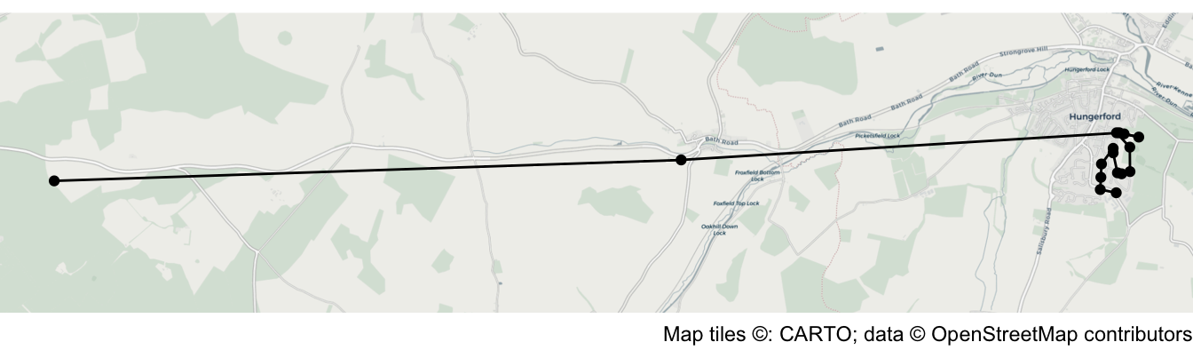

Map 16.3

Importantscale_x_continuous() vs scale_y_continuous()

The scale_y_continuous() function specifically controls the vertical (Y) axis of the map, so it only adds space above and below the data on the map. If we wanted to add space to the left and right of the data, we would need to use the scale_x_continuous() function. But in this case, since the map is already very wide relative to its height, we will not make the map any wider.

16.2.2 Adding arrows and curves

To add an arrow to the end of each line segment we can use the arrow() helper function from the ggplot2 package to specify the arrow argument of the geom_segment() function in our ggplot() stack. Here, we make the arrowhead smaller than the default by setting length = unit(3, "mm") and choose the style of the arrowhead with type = "closed".

To prevent the arrowheads from obscuring the points, we will give the points a thin white border by specifying shape = 21 (a circle with a separate border) and colour = "white", as well as making the points slightly bigger with size = 3.

Run this code in the R Console.

Code 16.6

R Console

ggplot() +
  # Add base map
  annotation_map_tile(type = "cartolight", zoomin = 0, progress = "none") +
  # Add lines between points
  geom_segment(
    aes(x = x_start, y = y_start, xend = x_end, yend = y_end),
    data = hungerford_lines,
    arrow = arrow(length = unit(3, "mm"), type = "closed"),
    colour = "darkorange4"
  ) +
  # Add points
  geom_point(
    aes(x = easting, y = northing),
    data = hungerford_shootings,
    shape = 21,
    colour = "white",
    fill = "darkorange4",
    size = 3
  ) +
  # Expand the map to show a larger area above/below the data
  scale_y_continuous(expand = expansion(2)) +
  # Specify coordinate system
  coord_sf(crs = "EPSG:27700") +
  # Add base map attribution statement
  labs(caption = "Map tiles ©: CARTO; data © OpenStreetMap contributors") +
  theme_void()

Map 16.4

This makes it easier to see that the shootings started at the point on the left of the map, but makes the problem of understanding the sequence of events in the town itself even worse. We will deal with this in Section 16.3.

In Map 16.4, we used the geom_segment() function to add the lines to our map. If we change this to geom_curve() the lines will become curved rather than straight. By specifying curvature = -0.2 we get a slightly straighter line than the default, and a left-hand curve because the value of curvature is negative. These curves show only the sequence in which the locations were visited. They do not show the route travelled between locations, which is not recorded in the data.

The other change we can make at this point is to add a layer of labels showing the order in which the shootings occurred. We don’t want the labels to overlap the points, so instead of adding labels with the geom_label() function from the ggplot2 package we will use geom_label_repel() from the ggrepel package that we learned about in Section 14.5. geom_label_repel() creates labels that are automatically offset from the points they relate to. For now, we will just label the first two locations.

At this point we can also make some minor changes to the map: adding a title and scale bar, putting a border around the map, and temporarily removing the base map attribution statement. The purpose of those changes will become clear in Section 16.3.

Add this code to the chapter_16.R script file and run it.

Code 16.7

chapter_16.R

# Make component maps ----------------------------------------------------------

# Create map showing overall locations of shootings
hungerford_map_overall <- ggplot() +
  # Plot base map
  annotation_map_tile(type = "cartolight", zoomin = 0, progress = "none") +
  # Plot lines between points
  geom_curve(
    aes(x = x_start, y = y_start, xend = x_end, yend = y_end),
    data = hungerford_lines,
    arrow = arrow(length = unit(3, "mm"), type = "closed"),
    curvature = -0.2,
    colour = "darkorange4"
  ) +
  # Add points
  geom_point(
    aes(x = easting, y = northing),
    data = hungerford_shootings,
    shape = 21,
    colour = "white",
    fill = "darkorange4",
    size = 3
  ) +
  # Add labels
  geom_label_repel(
    aes(x = easting, y = northing, label = order),
    data = filter(hungerford_shootings, order %in% 1:2),
    colour = "white",
    fill = "darkorange4",
    fontface = "bold",
    linewidth = 0
  ) +
  # Add scale bar
  annotation_scale(style = "ticks", line_col = "grey40", text_col = "grey40") +
  # Expand the map to show a larger area above/below the data
  scale_y_continuous(expand = expansion(2)) +
  # Specify coordinate system
  coord_sf(crs = "EPSG:27700") +
  # Add title
  labs(title = "Shootings in Wiltshire") +
  theme_void() +
  theme(
    panel.border = element_rect(colour = "grey20", fill = NA),
    plot.title = element_text(margin = margin(b = -18))
  )

Since we have saved this latest map to an object called hungerford_map_overall, we need to run the object name in the R Console in order to print the map in Positron’s Plots pane.

Code 16.8

R Console

hungerford_map_overall

Map 16.5

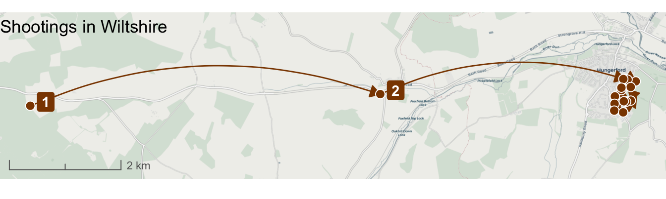
Now we have added arrowheads and curved lines, in Section 16.3 we will learn how to solve the problem of the events in the town itself being unclear on the map.

QuizMapping crime series

How can we show the sequence of locations in a crime series?

By adding street names to each location By removing locations that are too close together By connecting each point to the previous crime location By only mapping the final crime in the series

Why might we want to extend the area shown on a crime series map?

To include more contextual information about the surrounding environment To make the map appear more colourful To reduce the number of crime points displayed To increase the complexity of the visualisation

Which function in R can be used to prevent label overlap on crime maps?

theme_void() geom_label_repel() position_dodge() geom_text()

16.3 Multiple maps

Our existing map is difficult to understand because we have a mix of some events very close together (including several on the same street) and some that occurred further away. This means the closer events overlap on the map, especially now that we have made the points larger to distinguish them from the lines linking each event.

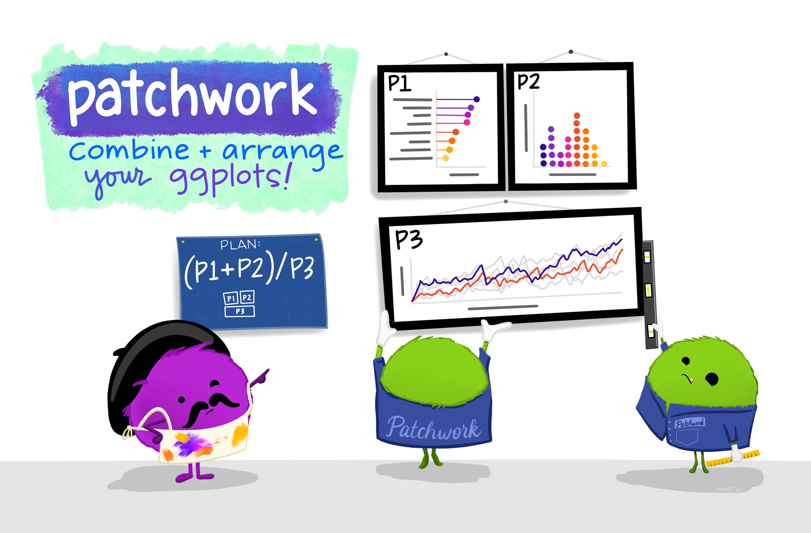
To deal with this problem we can display two maps: an overview map showing the whole area covered by the points and a detail map showing only the events in the town of Hungerford itself. In Section 15.5 we created small-multiple maps with facet_grid(), but what we want to do here is slightly different. In this case the maps show the same data at different scales, rather than different data for the same area. To combine these maps, we need to use the patchwork package, which can combine multiple maps or charts made using ggplot() into a single output.

We have already saved the overview map as hungerford_map_overall. We can create a detail map showing only the shootings in Hungerford itself by removing the first two points from hungerford_shootings (since they represent shootings outside the town itself). We can do this for all the existing layers using the slice() function from the dplyr package.

We will use the plot.margin argument to the theme() function to add a small amount of space at the top (and outside the border of) of this map. When we put the two maps together, that space will help separate the two maps. We will also get the map to cover a slightly larger area than it would by default by using the scale_x_continuous() and scale_y_continuous() functions.

Add this code to your script file and run it.

Code 16.9

chapter_16.R

# Create detail map showing shootings in Hungerford town
hungerford_map_town <- ggplot() +
  annotation_map_tile(type = "cartolight", zoomin = 0, progress = "none") +
  # Add lines between points
  geom_curve(
    aes(x = x_start, y = y_start, xend = x_end, yend = y_end),
    data = slice(hungerford_lines, 3:n()),
    arrow = arrow(length = unit(3, "mm"), type = "closed"),
    curvature = -0.2,
    colour = "darkorange4"
  ) +
  # Add points
  geom_point(
    aes(x = easting, y = northing),
    data = slice(hungerford_shootings, 3:n()),
    shape = 21,
    colour = "white",
    fill = "darkorange4",
    size = 3
  ) +
  # Add labels
  geom_label_repel(
    aes(x = easting, y = northing, label = order),
    data = slice(hungerford_shootings, 3:n()),
    colour = "white",
    fill = "darkorange4",
    fontface = "bold",
    linewidth = 0
  ) +
  # Add scale bar
  annotation_scale(style = "ticks", line_col = "grey40", text_col = "grey40") +
  # Expand the map to show a larger area around the data
  scale_x_continuous(expand = expansion(0.3)) +
  scale_y_continuous(expand = expansion(0.3)) +
  # Specify coordinate system
  coord_sf(crs = "EPSG:27700") +
  labs(title = "Shootings in Hungerford town") +
  theme_void() +
  theme(
    panel.border = element_rect(colour = "grey20", fill = NA),
    plot.margin = margin(t = 12)
  )

Code 16.10

R Console

hungerford_map_town

Map 16.6

Now we have two maps, we can use patchwork to combine them. The patchwork package uses mathematical operators to combine multiple ggplot2 objects. To place two plots beside one another, we would use the | operator. In this case we want to place one plot on top of another, so we use the / operator. You can combine plots in more-complicated ways by combining these operators, together with parentheses.

To position the town detail map (stored in hungerford_map_town) below the overview map (stored in hungerford_map_overall), we can use this code:

Code 16.11

R Console

hungerford_map_overall / hungerford_map_town

Map 16.7

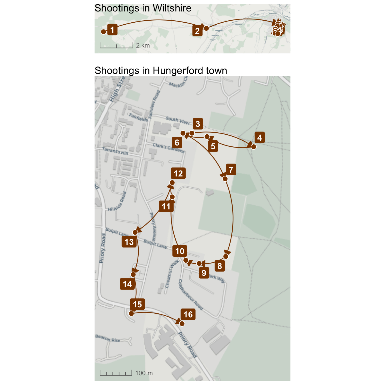
When we created the hungerford_map_overall object in Section 16.2.2, we gave the map title a negative margin using the plot.title argument to the theme() function. This had the effect of moving the title downwards onto the map to save space, since the top-left corner of the map was empty. We also added a scale bar, since when you present two related maps of different scales next to one another, it is useful to show the scales of both maps to help readers relate them to one another. You can see in Map 16.7, for example, the very different scales of the two maps.

We can add shared titles and captions to combined maps created with patchwork using the plot_annotation() function. We will add an overall title for the combined maps, as well as adding back the base map attribution statement, since it applies to both maps so there is no need to take up space by adding it to each map individually.

plot_annotation() also has a theme argument, which we can use to change the appearance of the shared title and caption just as we use theme() to change the appearance of elements on single maps. Finally, we can use ggsave() to save the combined map to an image file, as we learned to do in Section 7.10.

Add this code to the script file and run it.

Code 16.12

chapter_16.R

# Combine maps and add titles --------------------------------------------------

hungerford_map <- (hungerford_map_overall / hungerford_map_town) +
  plot_annotation(
    title = "Shootings during the Hungerford massacre",
    caption = str_glue(
      "Data from the official report into the shootings\nMap tiles ©: CARTO; ",
      "data © OpenStreetMap contributors"
    ),
    theme = theme(
      plot.caption = element_text(colour = "grey40", hjust = 0),
      plot.title = element_text(colour = "grey50", face = "bold", size = 14)
    )
  )

ggsave(
  here("output", "hungerford_map.jpg"),
  hungerford_map,
  width = 900 / 150,
  height = 900 / 150,
  dpi = 150
)

There are various other improvements that we could make to this map based on the mapping skills we have already learned during this course. For example, we could add the locations of buildings or particular facilities using data from OpenStreetMap. What information we choose to present on the map will depend on what information we think it is important to communicate to our audience.

The connecting curves should be interpreted cautiously. Their accuracy depends on the events being correctly linked and ordered, and they do not show the route travelled between locations.

QuizCombining maps

Why is it useful to combine an overview map with a detail map?

To show two unrelated datasets without explaining the connection To show the overall spatial pattern while preserving detail in a smaller area To avoid including scale information on either map To make every point appear at the same scale

Which patchwork operator places one plot above another?

The | operator The / operator The + operator The * operator

Why should both component maps include scale information?

Because patchwork requires every plot to contain one Because both maps always cover the same area Because the maps use different scales and readers need to interpret distance on each one Because scale bars identify the order of the events

16.4 Putting it all together

In this chapter, we practised how to:

• sort linked events into the correct order before mapping them;
• use lag() to associate each location with the previous location;
• connect locations using curves and directional arrows;
• expand the area displayed on a map;
• add labels that are automatically offset from their points with geom_label_repel();
• create overview and detailed maps; and
• combine multiple maps using the patchwork package.

When we are mapping crime data, it is important to remember that the rows in the data we are using often represent traumatic events that have happened to people. In this chapter, every row in the data represents one or more people who were killed or injured during the massacre. The people killed were Marcus Barnard, Roger Brereton, Francis Butler, Kenneth Clements, Victor Gibbs, Myrtle Gibbs, Susan Godfrey, Sandra Hill, Abdur Khan, Roland Mason, Sheila Mason, Ian Playle, Dorothy Ryan, Eric Vardy, Douglas Wainwright and George White.

The complete script in Code 16.13 contains everything needed to download the original data and make and save the composite map. Save chapter_16.R by pressing .

To check that the analysis is reproducible, restart R using the Restart R (⟳) button in Positron’s Console panel, then run the script from beginning to end.

Code 16.13

chapter_16.R

# This script creates a combination of maps showing the sequence of shootings
# during the Hungerford massacre in 1987

# Load data --------------------------------------------------------------------

# Load packages
pacman::p_load(ggrepel, ggspatial, here, httr2, patchwork, tidyverse)

# Download the original shootings data
request(
  "https://mpjashby.github.io/crimemappingdata/hungerford_shootings.csv"
) |>
  req_perform(path = here("data", "raw", "hungerford_shootings.csv"))

# Load the local copy of the shootings data
hungerford_shootings <- here("data", "raw", "hungerford_shootings.csv") |>
  read_csv() |>
  arrange(order)


# Prepare data -----------------------------------------------------------------

# Create dataset of lines joining shootings in sequence
hungerford_lines <- hungerford_shootings |>
  # Arrange the rows in order of the sequence of shootings
  arrange(order) |>
  # Make it clear the coordinates refer to the coordinates we want to use for
  # the *end* of each line, to distinguish them from the second set of
  # coordinates we'll create next
  rename(x_end = easting, y_end = northing) |>
  # Copy the coordinates from the row above each row to create a second set of
  # coordinates for the *start* of each line
  mutate(x_start = lag(x_end), y_start = lag(y_end)) |>
  # Remove the first row, which now contains missing values for `y_start` and
  # `x_start`, and which we don't need
  drop_na(x_start, y_start)


# Make component maps ----------------------------------------------------------

# Create map showing overall locations of shootings
hungerford_map_overall <- ggplot() +
  # Plot base map
  annotation_map_tile(type = "cartolight", zoomin = 0, progress = "none") +
  # Plot lines between points
  geom_curve(
    aes(x = x_start, y = y_start, xend = x_end, yend = y_end),
    data = hungerford_lines,
    arrow = arrow(length = unit(3, "mm"), type = "closed"),
    curvature = -0.2,
    colour = "darkorange4"
  ) +
  # Add points
  geom_point(
    aes(x = easting, y = northing),
    data = hungerford_shootings,
    shape = 21,
    colour = "white",
    fill = "darkorange4",
    size = 3
  ) +
  # Add labels
  geom_label_repel(
    aes(x = easting, y = northing, label = order),
    data = filter(hungerford_shootings, order %in% 1:2),
    colour = "white",
    fill = "darkorange4",
    fontface = "bold",
    linewidth = 0
  ) +
  # Add scale bar
  annotation_scale(style = "ticks", line_col = "grey40", text_col = "grey40") +
  # Expand the map to show a larger area above/below the data
  scale_y_continuous(expand = expansion(2)) +
  # Specify coordinate system
  coord_sf(crs = "EPSG:27700") +
  # Add title
  labs(title = "Shootings in Wiltshire") +
  theme_void() +
  theme(
    panel.border = element_rect(colour = "grey20", fill = NA),
    plot.title = element_text(margin = margin(b = -18))
  )

# Create detail map showing shootings in Hungerford town
hungerford_map_town <- ggplot() +
  annotation_map_tile(type = "cartolight", zoomin = 0, progress = "none") +
  # Add lines between points
  geom_curve(
    aes(x = x_start, y = y_start, xend = x_end, yend = y_end),
    data = slice(hungerford_lines, 3:n()),
    arrow = arrow(length = unit(3, "mm"), type = "closed"),
    curvature = -0.2,
    colour = "darkorange4"
  ) +
  # Add points
  geom_point(
    aes(x = easting, y = northing),
    data = slice(hungerford_shootings, 3:n()),
    shape = 21,
    colour = "white",
    fill = "darkorange4",
    size = 3
  ) +
  # Add labels
  geom_label_repel(
    aes(x = easting, y = northing, label = order),
    data = slice(hungerford_shootings, 3:n()),
    colour = "white",
    fill = "darkorange4",
    fontface = "bold",
    linewidth = 0
  ) +
  # Add scale bar
  annotation_scale(style = "ticks", line_col = "grey40", text_col = "grey40") +
  # Expand the map to show a larger area around the data
  scale_x_continuous(expand = expansion(0.3)) +
  scale_y_continuous(expand = expansion(0.3)) +
  # Specify coordinate system
  coord_sf(crs = "EPSG:27700") +
  labs(title = "Shootings in Hungerford town") +
  theme_void() +
  theme(
    panel.border = element_rect(colour = "grey20", fill = NA),
    plot.margin = margin(t = 12)
  )


# Combine maps and add titles --------------------------------------------------

hungerford_map <- (hungerford_map_overall / hungerford_map_town) +
  plot_annotation(
    title = "Shootings during the Hungerford massacre",
    caption = str_glue(
      "Data from the official report into the shootings\nMap tiles ©: CARTO; ",
      "data © OpenStreetMap contributors"
    ),
    theme = theme(
      plot.caption = element_text(colour = "grey40", hjust = 0),
      plot.title = element_text(colour = "grey50", face = "bold", size = 14)
    )
  )

ggsave(
  here("output", "hungerford_map.jpg"),
  hungerford_map,
  width = 900 / 150,
  height = 900 / 150,
  dpi = 150
)

16.5 Further reading

• The Crime Linkage International NetworK provides information about research and practice in behavioural case linkage.
• The official patchwork documentation includes further examples of arranging and annotating multiple plots.

Photograph of PC Roger Brereton’s funeral from Berkshire Live, artwork by Allison Horst.

QuizCheck your knowledge: Revision questions

Answer these questions to check you have understood the main points covered in this chapter. Write between 50 and 100 words to answer each question.

1. What is a crime series, and in what circumstances might mapping a series provide information that would not be visible if each crime were considered separately?
2. What challenges do investigators face when trying to determine whether crimes are linked?
3. Why is it useful to visualise a crime series on a map? Give some examples of when a map of a crime series might be useful.
4. Explain the role of arrows and labels in mapping crime series. How do these elements help improve the clarity of crime maps?
5. Describe the steps taken to prepare a dataset for mapping a crime series in R. Why is it necessary to create a dataset of linked points?