9  Mapping area data

In this chapter, we will learn how to create crime maps that display data for geographic areas rather than individual crime locations. We will explore how to count crimes within predefined areas, visualize these counts using thematic maps, and understand the challenges of interpreting area-based data. We will also explore interactive maps, crime rate calculations, and important spatial concepts like the ecological fallacy.

TipBefore you start

1. Open Positron or – if you already have Positron open – start a new R session by clicking the Restart R (⟳) button in the Console panel. This makes sure no code you ran previously will interfere with the work you do in this chapter.
2. Make sure you are working in the crime mapping project workspace you created in Section 1.5. In the top-right corner of the Positron window, you should see a folder icon and the words crime_mapping. If not, click the File menu, then Open Folder … and choose the crime_mapping folder.

9.1 Introduction

In Chapter 5 we produced a point map showing the locations of individual crimes, and in Section 6.2 we produced a density map showing patterns derived from those individual points. Data that includes the locations of individual crimes is sometimes known as point data because we know the point in space at which each crime occurred.

Map 9.1

Another type of crime data is area data. The most common type of area data used for crime mapping is data that does not include the locations of individual crimes but instead consists of counts of the number of crimes occurring in one or more areas. Maps of area data can be useful for several purposes:

• We might want to compare the number of crimes in different areas, such as police districts, to decide which district to allocate extra funds to.
• We might want to estimate the relative risk of a crime occurring in different areas by calculating crime rates using counts of crimes and population data.
• We might only have been given access to counts of crimes for different areas, rather than the location of each crime, perhaps in order to protect the privacy of crime victims.

In all these cases we need to make maps of crimes for areas, rather than showing the locations of individual crimes or the density of crimes generated from datasets of individual crime locations. A map in which areas are shaded according to data values is called a choropleth map (in English, ‘choropleth’ is usually pronounced ‘kor-o-pleth’). A choropleth map is one type of thematic map.

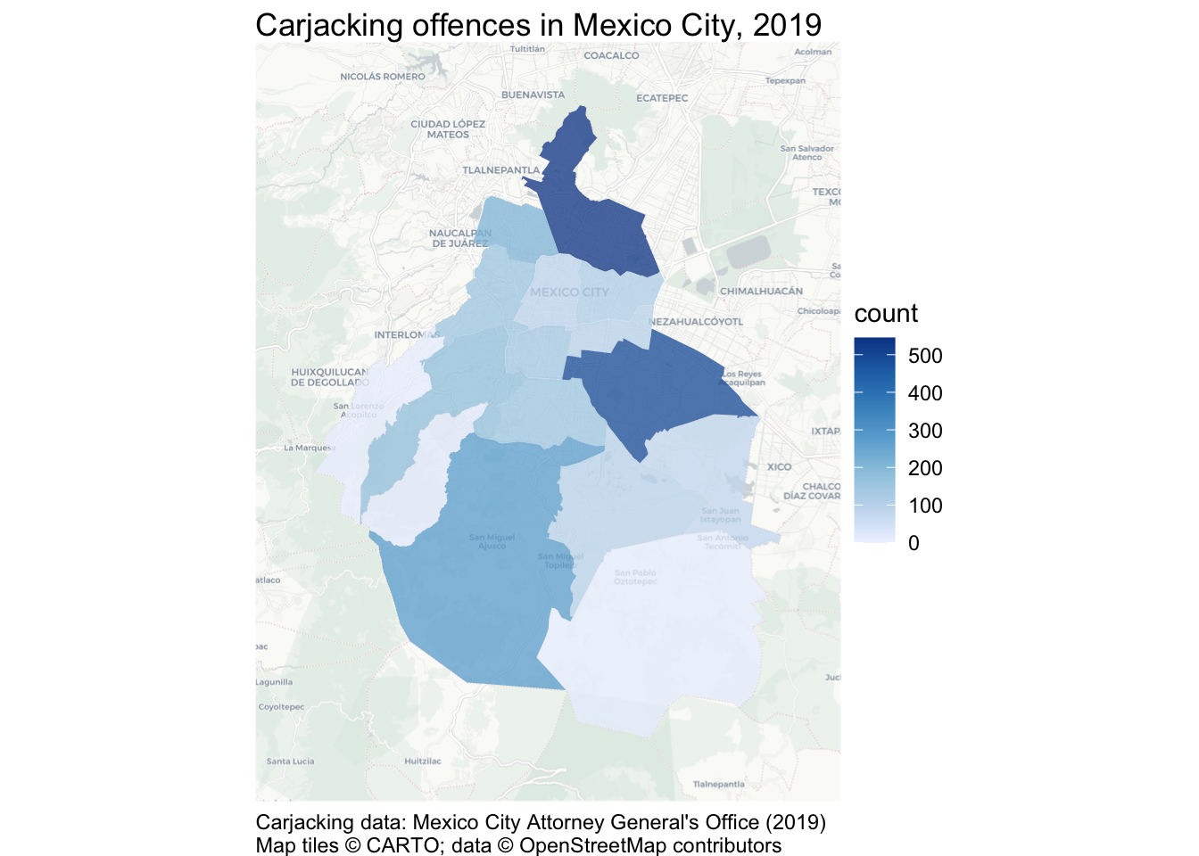
In the first analysis in this chapter, you will produce this map of carjacking offences in Mexico City:

Map 9.2

In this chapter, we will learn how to:

• count points within predefined areas using hotspot_count();
• create static and interactive choropleth maps;
• join tabular data to area boundaries and check the result;
• calculate and map crime rates;
• distinguish incidence, prevalence and concentration rates; and
• recognise the ecological fallacy and the modifiable areal unit problem.

The process we will use has three main stages:

Load

source data

Wrangle

e.g. count points or join datasets

Visualise

counts or rates using a static or interactive choropleth map

ImportantDon’t create area maps unless you need to

Do not aggregate point-level crime data to counts of crimes for areas unless you have a good reason to do so.

Choropleth maps have several shortcomings that we will look at in this chapter. If you have data on the locations of individual crimes then you should typically present those either as individual points (if there are only a few crimes) or using a kernel density map. If you have point-level crime data, you should only use a choropleth map if you need to compare administrative areas or because you want to calculate crime risk and you only have population data for areas.

9.2 Counting crimes

Sometimes we will want to know how many crimes have occurred in different formal areas within a city. For example, we might want to know how many crimes of a particular type had occurred in each neighbourhood in a city as part of a review of the performance of different police teams, or to decide which neighbourhoods should be given more crime-prevention funding.

To calculate counts of crimes for areas, we need

1. a dataset representing the crime locations and
2. a dataset representing the boundaries of the areas that we want to calculate counts for.

In this chapter, we will count how many carjacking offences occurred in each alcaldía (borough) of Mexico City in 2019. The result will be an SF object containing the outline of each borough and its carjacking count:

municip	nomgeo	n
9	Milpa Alta	13
14	Benito Juárez	140
5	Gustavo A. Madero	545
3	Coyoacán	152
16	Miguel Hidalgo	152
8	La Magdalena Contreras	21

TipWhat is carjacking?

Carjacking is robbery in which a vehicle is stolen using violence or the threat of violence. It differs from other types of vehicle theft because it involves taking the vehicle from the owner while they are using it, rather than breaking into a vehicle that has been left unattended. Because carjacking involves violence, it is considered more serious than other vehicle-related theft.

Find out more about carjacking

9.2.1 Load the data

Create a new R script in Positron and save it as chapter_09a.R in the R folder. Write a comment at the top explaining that the script will show the number of carjacking offences in each alcaldía in Mexico City in 2019. Keep all the permanent code for this first analysis in this file.

Add a line to the script file (with an appropriate comment above it) to load the here, httr2, sf, sfhotspot and tidyverse packages. If you need help with that code, look back to Section 2.3.1.

We need two datasets for this script: a dataset of carjackings and one of alcaldía boundaries. First download both original files into data/raw, then load the local files. Keeping the source files in data/raw makes the analysis easier to repeat and ensures that we do not accidentally edit the original data.

https://mpjashby.github.io/crimemappingdata/cdmx_car_jacking.gpkg

In your script file, write the code needed to download this dataset, then load it into an object called cdmx_car_jacking (CDMX is a common Spanish-language abbreviation for Mexico City, short for Ciudad de México).

When you are writing this code, think about what sort of file you are trying to load and which function you should use to do it. If you need help, look at Appendix A. Make sure your code has comments that explain what it does.

Now write the code needed to download this dataset, then load it and store it in an object called cdmx_alcaldias:

https://mpjashby.github.io/crimemappingdata/cdmx_alcaldias.gpkg

Once you have written the code to load the packages and data, click the Solution button below to check your code.

Code 9.1

chapter_09a.R

# This script counts carjacking offences in each alcaldía in Mexico City in
# 2019 and produces a choropleth map of those counts.

# Load packages
pacman::p_load(here, httr2, sf, sfhotspot, tidyverse)

# Download the raw data
request(
  "https://mpjashby.github.io/crimemappingdata/cdmx_car_jacking.gpkg"
) |>
  req_perform(path = here("data", "raw", "cdmx_car_jacking.gpkg"))

request(
  "https://mpjashby.github.io/crimemappingdata/cdmx_alcaldias.gpkg"
) |>
  req_perform(path = here("data", "raw", "cdmx_alcaldias.gpkg"))

# Load carjacking and alcaldía data
cdmx_car_jacking <- here("data", "raw", "cdmx_car_jacking.gpkg") |>
  read_sf()

cdmx_alcaldias <- here("data", "raw", "cdmx_alcaldias.gpkg") |>
  read_sf()

9.2.2 Count crimes in each borough

Now that we have loaded our data, the next step is to count the number of offences in each borough and produce an R object that contains the boundaries of the boroughs together with the number of offences in each one. We can use the hotspot_count() function from the sfhotspot package to do this.

By default, hotspot_count() produces counts of points in cells in a grid (we saw this when we used hotspot_kde() in Chapter 6). This is often useful, but in this case we instead want to produce a count for each alcaldía. To do that, we can pass the cdmx_alcaldias object to the grid argument of hotspot_count(). Add this code to your script file:

Code 9.2

chapter_09a.R

# Count carjacking offences in each alcaldía
car_jacking_counts <- hotspot_count(cdmx_car_jacking, grid = cdmx_alcaldias)

Run this code now. When you run it, you will see warnings appear in the R Console:

Warning in hotspot_count(cdmx_car_jacking, grid = cdmx_alcaldias): `data` has points with the co-ordinates "0, 0".
ℹ This usually indicates a problem with the data.
ℹ Check co-ordinates are correct (e.g. by mapping them).

Warning: 152 point is outside the area covered by the supplied polygons.

This means that some of the points in the cdmx_car_jacking object are outside the area covered by the cdmx_alcaldias object. This is a common issue with crime data. Sometimes the authorities for an area (e.g. the police agency for a city) will record a small number of crimes that occurred outside their area of responsibility if they are linked to a larger series of crimes they are investigating. On other occasions points will appear outside the area we would expect due to processing errors.

If any error happened before you were given the data, there is probably little you can do to fix it. But it is still important to check to make sure you understand why there is a problem with the data. We can usually do that by producing a very basic map showing the data we are using on a base map.

Run this code in the R Console:

Code 9.3

R Console

hotspot_map(cdmx_car_jacking)

Map 9.3

This map shows that the points in the cdmx_car_jacking dataset are located in two parts of the world, which is not what we would expect. Some points appear in Mexico as we would expect, but some appear in the Gulf of Guinea off the coast of West Africa. These points are located on ‘Null Island’, which we will learn more about in Section 10.3.4.

There are 152 points outside the boundary of Mexico City out of 2,811 in total (5.4%). All these points are excluded from the borough counts. We can continue with this example, but we should document the exclusion rather than assuming it has no effect. In a real analysis, we would also investigate how the errors arose and whether excluded records differ systematically from the records with valid locations.

QuizCounting crimes

Which of the following is not a common reason why crime analysts might choose to count the number of crimes in different areas?

To combine crime counts with other data that is only available for pre-set areas, e.g. population data Because point crime data is inherently unreliable Because it is often useful for police to know how many crimes occurred in different administrative areas To understand how counts of crimes in an area change over time

What is a choropleth map?

A map that uses shading to represent data values across different areas A map that shows individual points for crime locations A 3D model of crime distribution A type of bar chart

Which of the following is not a reason some crime locations might be recorded outside the area covered by the agency doing the crime recording?

Errors in data recording Errors in data processing All incidents in a crime series being recorded by one agency, wherever each incident occurred To preserve victim privacy

9.3 Mapping areas

Maps showing data (such as counts of crimes) for different areas are extremely common in all types of spatial analysis. Watch this video for an introduction to some of the issues you should be aware of when mapping areas.

TranscriptVideo transcript: We need to talk about boundaries

I’m standing in a Suburban Street in Southwest London or at least that side of the street is in London that side of the street is in the county of Sur outside London the outer boundary of London divides one side of this street from the other that has all sorts of consequences for the residents on both sides residents on the Su side pay about 10% more in property taxes than those on the London side older people living on the London side get to travel free on underground trains while those living on

the S side don’t and if you call an ambulance to an address on one side of the street a different Ambulance Service responds than would respond on the other side apart from all those practical differences the fact that the London boundary divides this neighborhood in half is important when it comes to showing data about areas on maps we often show data for areas on a type of map called a COR pleth map where each area for which we have data is represented by a polygon and the color

of the polygon shows a value from the data so for example on this map darker Shades represent higher levels of Health inequality and lighter Shades represent lower levels lots of statistical data is published for Geographic areas rather than for individual addresses or streets so if you want to know about poverty in this area or health or any number of other things you’ll be able to find data for different areas that contain this street but you typically won’t find data for the street itself that’s because some streets have only a few houses on

them so publishing data at address or street level would risk breaching the privacy of the people who live here agencies that publish data about places have to choose which areas they publish data for for example the government publishes estimates of poverty in each local government Ward then also Aggregates that data into estimates of poverty at local Authority level and at Regional level and at National level publishing data for administrative areas like Wards buroughs and regions is useful for lots of reasons for example it could help a local counselor

understand problems their own Ward might face but one issue with administrative areas is that their boundaries tend to change every few years to reflect changes in population that makes it difficult to answer questions about how things like poverty have changed over time to get around this problem governments tend to also publish data for a set of statistical areas that change much less often like the administrative areas there are typically several nested levels of statistical area in England for example statistical data is published for small areas called

output areas which are then grouped into progressively larger areas with data sets being published for areas at each level statistical data for local areas can tell us a lot about these places but there is one problem we need to be aware of this is called the ecological fallacy the problem here is that when we look at maps that show data for different areas our brains tend to assume that the data shown for a particular area applies equally to every street house or person in that area equally when there’s a

difference between two areas on a map we tend to assume that the difference happens at the boundary between those areas this is a problem because in fact it’s quite likely that places just one side of the boundary or the other tend to be pretty similar to each other despite looking quite different on a corle map so whenever we look at a map that shows data for areas we need to remember that the data only represents a summary of each area as a whole rather than telling us something about any

particular Street or place within that area because of the ecological fallacy we generally avoid using corle maps to show data that we could show in a more detailed way for example it’s almost always better to show hotpots of crime using a density map rather than a chop plma but sometimes we have little choice but to use a corpath map because data is only available for areas not in individual locations so in summary lots of useful data is published for areas rather than individual streets or addresses governments typically publish

data for both administrative and statistical areas and whenever we use a corop map we need to consider the ecological fallacy

Because so much of the data that we might use in crime mapping is only available for pre-defined areas, we often have no choice about which areas to use. But whether we choose the areas or not, area data can only tell us about each area as a whole. It cannot tell us that every person or place within an area has the area’s average characteristics.

Drawing a conclusion about individuals from data that describes groups or areas is known as the ecological fallacy. For example, a map might show that boroughs with more poverty have higher crime rates, but that does not prove that the people who experience poverty are the people committing those crimes. The map describes relationships between boroughs, not relationships between individuals.

QuizMapping areas

What is a choropleth map?

A map that shows streets and buildings in high detail A map where areas are shaded to represent different values of data A map that shows individual data points for each incident A map that shows only statistical areas, not administrative boundaries

Why is statistical data often published for areas rather than individual streets?

It is more accurate at the local level It allows emergency services to respond more quickly It helps ensure the privacy of individuals It reduces the cost of data collection

What is the ecological fallacy?

Drawing a conclusion about individuals from data that describes an area as a whole The assumption that environmental factors affect statistical data The assumption that all choropleth maps are inaccurate The assumption that larger areas always contain more people

What is the key mistake people often make when interpreting choropleth maps?

They believe that the maps are drawn inaccurately They ignore differences in shading They assume all data is outdated They assume that boundaries between areas reflect sharp differences in data

ImportantArea data cannot describe individuals

The ecological fallacy is an error in how we interpret data, rather than something that every choropleth map automatically commits. Nevertheless, choropleth maps create a particular risk of this error because they visually emphasise differences between whole areas. Whenever we plan to use a choropleth map, it is worth asking whether another type of map would represent the data more effectively.

Nevertheless, in some circumstances a choropleth map will be the best choice either because we only have data for pre-defined areas or because we are specifically interested in comparing areas (e.g. in working out if there is more crime in one neighbourhood or police district than another).

9.3.1 Boundaries can change the pattern

The pattern shown on a choropleth map also depends on the boundaries used to divide the study area. If the same point data were counted using neighbourhoods, police districts or a regular grid, each set of areas would group the points differently and could produce a different-looking pattern. Results can also change when small areas are combined into larger ones.

This is known as the modifiable areal unit problem (MAUP). It has two related parts:

• the scale effect: results change when we use larger or smaller areas; and
• the zoning effect: results change when boundaries are drawn in different places, even if the areas remain roughly the same size.

The MAUP cannot be removed from an analysis that uses area data. We should therefore explain which boundaries we used, avoid treating them as natural divisions between communities and, where possible, check whether our conclusions change when we use a different set of areas.

QuizThe modifiable areal unit problem

What does the modifiable areal unit problem mean for a choropleth map?

It proves that choropleth maps should never be used It occurs only when boundary data contain errors A spatial pattern can change when the same data are grouped using different boundaries It means every person in an area has the same level of risk

We have already loaded the data we need to create a map of carjackings in Mexico City, and counted how many offences occurred in each alcaldía. Since we used hotspot_count() from the sfhotspot package to count the offences, we can use hotspot_map() to create a map of the counts. Add this code to your script file and run it.

Code 9.4

chapter_09a.R

# Create a choropleth map of carjacking counts
car_jacking_map <- hotspot_map(
  car_jacking_counts,
  basemap_type = "cartolight",
  caption = "Carjacking data: Mexico City Attorney General's Office (2019)"
) +
  labs(title = "Carjacking offences in Mexico City, 2019")

car_jacking_map

Map 9.4

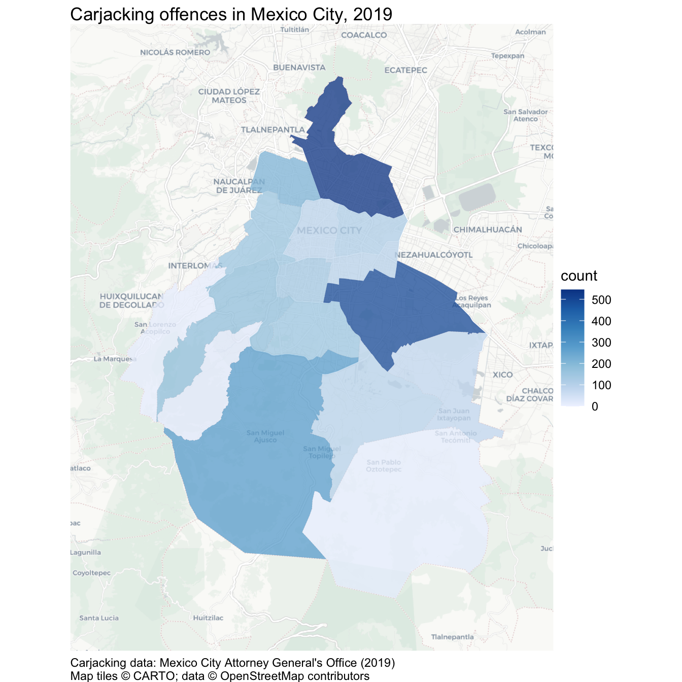
We could build on this map in several ways. For example, in Section 9.5 we will learn how to show crime rates on a map, as an alternative to crime counts. But in Section 9.4, we will learn how to make interactive crime maps.

Your complete script for this analysis should now look like this:

Code 9.5

chapter_09a.R

# This script counts carjacking offences in each alcaldía in Mexico City in
# 2019 and produces a choropleth map of those counts.

# Load packages
pacman::p_load(here, httr2, sf, sfhotspot, tidyverse)

# Download the raw data
request(
  "https://mpjashby.github.io/crimemappingdata/cdmx_car_jacking.gpkg"
) |>
  req_perform(path = here("data", "raw", "cdmx_car_jacking.gpkg"))

request(
  "https://mpjashby.github.io/crimemappingdata/cdmx_alcaldias.gpkg"
) |>
  req_perform(path = here("data", "raw", "cdmx_alcaldias.gpkg"))

# Load carjacking and alcaldía data
cdmx_car_jacking <- here("data", "raw", "cdmx_car_jacking.gpkg") |>
  read_sf()

cdmx_alcaldias <- here("data", "raw", "cdmx_alcaldias.gpkg") |>
  read_sf()

# Count carjacking offences in each alcaldía

car_jacking_counts <- hotspot_count(cdmx_car_jacking, grid = cdmx_alcaldias)

# Create a choropleth map of carjacking counts

car_jacking_map <- hotspot_map(
  car_jacking_counts,
  basemap_type = "cartolight",
  caption = "Carjacking data: Mexico City Attorney General's Office (2019)"
) +
  labs(title = "Carjacking offences in Mexico City, 2019")

car_jacking_map

Save chapter_09a.R by pressing . Keep this script in the R folder and the original downloaded files in data/raw.

9.4 Making an interactive map

So far in this course, all the maps we have made using hotspot_map() have been static images. These are useful for lots of different circumstances, and are usually the only choice if we want to produce a written report as a Word document or PDF. But in some circumstances it may be useful to produce a map that you can interact with by zooming in or panning around different areas. This can be useful when readers might want to look at areas of the map in more detail than is possible without zooming in.

In this section we will make an interactive map of counts of murders in each district in the state of Uttar Pradesh in northern India in 2014. Uttar Pradesh is India’s most populous state, with more than 200 million residents.

9.4.1 Combining datasets

Restart R using the Restart R (⟳) button in Positron’s Console panel. Create a new R script and save it as chapter_09b.R in the R folder. Keep all the permanent code for the Uttar Pradesh analysis in this file.

Paste Code 9.6 into chapter_09b.R, then run it by pressing followed by . The code downloads copies of the source data into data/raw, then loads those local files.

Code 9.6

chapter_09b.R

# This script produces interactive maps of murder counts and murder rates in
# districts in Uttar Pradesh, India, in 2014.

# PREPARE ----------------------------------------------------------------------

# Load packages
pacman::p_load(here, httr2, leaflet, sf, tidyverse)

# Download the raw murder-count and district-boundary data
request(
  "https://mpjashby.github.io/crimemappingdata/uttar_pradesh_murders.csv"
) |>
  req_perform(path = here("data", "raw", "uttar_pradesh_murders.csv"))

request(
  "https://mpjashby.github.io/crimemappingdata/uttar_pradesh_districts.gpkg"
) |>
  req_perform(path = here("data", "raw", "uttar_pradesh_districts.gpkg"))

# Load murder counts and district boundaries
murders <- here("data", "raw", "uttar_pradesh_murders.csv") |>
  read_csv(show_col_types = FALSE)

districts <- here("data", "raw", "uttar_pradesh_districts.gpkg") |>
  read_sf()

You can see from this code that we are loading two datasets:

• a CSV file called uttar_pradesh_murders.csv containing counts of murders in each district, and
• a geopackage file called uttar_pradesh_districts.gpkg containing the boundaries of each district.

The murder counts were published by the Government of India, while the boundary data were compiled by Hindustan Times Labs. Identifying the organisations responsible for source data helps readers assess how the data were produced and what limitations they may have.

To start, let’s look at the two datasets in the R Console:

Code 9.7

R Console

head(murders)

# A tibble: 6 × 2
  district       murder
  <chr>           <dbl>
1 Agra              178
2 Aligarh           179
3 Allahabad         132
4 Ambedkar Nagar     24
5 Amethi             36
6 Amroha             60

Code 9.8

R Console

head(districts)

Simple feature collection with 6 features and 2 fields
Geometry type: POLYGON
Dimension:     XY
Bounding box:  xmin: 77.42308 ymin: 24.80419 xmax: 82.35455 ymax: 28.90105
Geodetic CRS:  WGS 84
# A tibble: 6 × 3
  state         district_name                                               geom
  <chr>         <chr>                                              <POLYGON [°]>
1 Uttar Pradesh Agra          ((77.6444 27.23444, 77.65405 27.23463, 77.65336 2…
2 Uttar Pradesh Bareilly      ((78.97474 28.41527, 78.97981 28.41454, 78.98546 …
3 Uttar Pradesh Etah          ((79.20766 27.56734, 79.20418 27.56314, 79.19801 …
4 Uttar Pradesh Shahjahanpur  ((80.30972 28.46321, 80.29755 28.46668, 80.28367 …
5 Uttar Pradesh Pilibhit      ((79.67865 28.84923, 79.67203 28.83937, 79.67553 …
6 Uttar Pradesh Allahabad     ((81.54684 25.1848, 81.55587 25.1857, 81.5577 25.…

This output shows us that both datasets include a column that contains the name of each district in Uttar Pradesh. In the murders dataset that column is called district while in the districts dataset that column is called district_name. We can also see that only the murders object contains a count of murders in each district (in the murder column) and only the districts object contains the outlines of each district boundary (in the geom column). To make a choropleth map of the murder counts, we will need to join the two datasets so we have a single SF object that contains all the data we need.

There are several ways to join data in R. In this case, we want to join the two datasets based on the value of a column in both datasets that stores the same information (in this case, the district names). To do that we use the left_join() function, one of a family of joining functions in the dplyr package that join two objects together based on the values of particular columns.

To understand how left-joins work, imagine we had two datasets called x and y:

Dataset x

key	x_value
1	x1
2	x2
3	x3

Dataset y

key	y_value
1	y1
2	y2
4	y4

We could use left_join(x, y) to merge them into one combined dataset. This function has left in the name because it joins the two datasets by adding matching rows from the right-hand dataset (y) to each row in the left-hand dataset (x). The result would be:

Result of left_join(x, y)

key	x_value	y_value
1	x1	y1
2	x2	y2
3	x3	NA

The result produced by left_join() always includes all the rows from x and the matching rows from y. There isn’t a row in y for which the value in the key column is 3, so y_value for that row in the result is missing (NA). Key 4 appears only in y and not in x, so it is not included in the result.

In our case, we want the combined dataset to include exactly one row for each district in districts. Since we want to keep all those rows, we use districts as the first argument to left_join(), i.e. left_join(districts, murders). If a district has no matching row in murders, the resulting murder count will be NA. This means “no matching information”, not automatically “zero murders”. We should only replace that value with zero if the data documentation confirms that omitted districts represent genuine zero counts.

By default, left_join() will match the rows in the districts and murders objects using all the column names that are present in both datasets. This can sometimes have unexpected results, so it is safer to specify which columns we want to match to be based on using the by argument to left_join(). There are lots of ways we could join two datasets, so we will use the join_by() helper function to assist with this.

Copy this code into your script file and run it.

Code 9.9

chapter_09b.R

# WRANGLE ----------------------------------------------------------------------

# Join murder counts to district boundaries
district_murders <- left_join(
  districts,
  murders,
  by = join_by(district_name == district)
)

Note that, similar to the filter() function, we use the == operator here to specify that we want the rows to be matched if the value of the district_name column in districts is the same as the value of the district column in murders.

To check the result produced by this code, run head(district_murders) in the R Console. The output should look like this:

Simple feature collection with 6 features and 3 fields
Geometry type: POLYGON
Dimension:     XY
Bounding box:  xmin: 77.42308 ymin: 24.80419 xmax: 82.35455 ymax: 28.90105
Geodetic CRS:  WGS 84
# A tibble: 6 × 4
  state         district_name                                        geom murder
  <chr>         <chr>                                       <POLYGON [°]>  <dbl>
1 Uttar Pradesh Agra          ((77.6444 27.23444, 77.65405 27.23463, 77.…    178
2 Uttar Pradesh Bareilly      ((78.97474 28.41527, 78.97981 28.41454, 78…    132
3 Uttar Pradesh Etah          ((79.20766 27.56734, 79.20418 27.56314, 79…     65
4 Uttar Pradesh Shahjahanpur  ((80.30972 28.46321, 80.29755 28.46668, 80…     88
5 Uttar Pradesh Pilibhit      ((79.67865 28.84923, 79.67203 28.83937, 79…     54
6 Uttar Pradesh Allahabad     ((81.54684 25.1848, 81.55587 25.1857, 81.5…    132

If you want to view the whole dataset, run view(district_murders) in the R Console instead. You can see that district_murders contains all the columns from the districts object and the murder column from the murders dataset. It does not contain the district column from the murders dataset, since this has been merged into the existing district_name column.

Joining datasets in any programming language (or even using functions like VLOOKUP() in Microsoft Excel) can be complicated. It is particularly important that you understand in each case (a) which dataset you are going to merge data into (in this case, districts), (b) which dataset columns are going to be taken from (in this case, murders) and (c) which columns are going to be used as the basis for the join (in this case, district_name and district). Thinking through what you are trying to achieve before writing the code will prevent many problems later.

ImportantAlways check a join

left_join() warns about some potential problems that might occur when joining two datasets, but it does not detect every mistake. An unmatched row can produce NA without any warning. After every join, check:

• whether the result has the expected number of rows;
• whether the joining columns contain duplicate values; and
• whether important columns contain unexpected missing values.

For the current data, the result has 75 rows (one for each district), no duplicated district names and no missing murder counts. If you receive a warning or a check gives an unexpected result, investigate it before continuing. See Chapter 8 if you need help dealing with warnings produced by R code.

NoteOptional: attaching area information to individual crimes

hotspot_count() gives us one row per area, with the number of crimes in each area. Sometimes we instead want to join two spatial datasets but keep one row per crime and add information about the area in which it occurred. For example, we might want to attach borough names to records of individual crimes, based on the borough in which the crime happened. A spatial join can do this.

Whereas left_join() matches values in columns, st_join() from the sf package matches features by their locations. For example, run this code in the R Console to attach borough names to the carjacking points we loaded earlier:

Code 9.10

R Console

car_jacking_boroughs <- cdmx_car_jacking |>
  st_transform(st_crs(cdmx_alcaldias)) |>
  st_join(select(cdmx_alcaldias, nomgeo))

Both objects must use the same coordinate reference system, so we use st_transform() before joining them. The result keeps the crime-point geometry and adds the nomgeo column containing borough names. By default, st_join() matches features that intersect: a point inside an area or on its boundary matches that area.

Unmatched crimes remain in the result with a missing (NA) borough name. A crime that matches more than one area appears in more than one row, for example if it lies on a shared boundary. Check the row counts and missing names before using the result, and investigate unexpected matches rather than simply deleting duplicate rows.

Use hotspot_count() when you need area counts. Use st_join() when you need area attributes attached to individual records, for example to compare the characteristics of crimes in different boroughs.

9.4.2 Interactive choropleth maps

Data visualisations (including maps) in R are made using the ggplot2 package, sometimes in combination with specialist helper functions (such as hotspot_map()) for particular types of visualisation. But interactive maps are made using a different package: leaflet. The functions in the leaflet package work in a similar way to ggplot2, but with a few differences.

To make maps with leaflet, we create a stack of functions in a similar way to the stacks we have already created by combining functions from the ggplot2 package with hotspot_map(). Note that while the concept of a stack is similar, we cannot use functions from the ggplot2 package in a leaflet stack, or vice versa. Also, we construct leaflet stacks using the pipe operator |> rather than the plus operator + that we use in ggplot2.

We can create a very basic leaflet map using the leaflet() function to create the stack, the addProviderTiles() function to add a base map and the addPolygons() function to add the district outlines. We have already loaded the leaflet package in our script file, so we can run this code in the R Console to create our first interactive map.

Code 9.11

R Console

# Create interactive map
leaflet(district_murders) |>
  # Add base map
  addProviderTiles("OpenStreetMap.Mapnik") |>
  # Add district polygons
  addPolygons(fillOpacity = 0.75)

Map 9.5

You can interact with this map by clicking the buttons to zoom in and out, and by moving around the map area. For example, you can zoom out to see where Uttar Pradesh is relative to other places, or zoom in to see where particular cities are within Uttar Pradesh. This could be very useful in helping people understand the context of crime data.

In this map we use the ‘OpenStreetMap.Mapnik’ style of base map, but leaflet can use a large number of different base maps that you can view in this online gallery.

However, this map isn’t very useful for understanding murders in Uttar Pradesh because it doesn’t show how many murders there were in each district. To do that, we need to specify that each district should be coloured according to the values in the murder column of the district_murders object. With a map created by combining ggplot2 functions with hotspot_map(), we would do this with a function such as scale_fill_distiller() (see Section 7.6), but with a leaflet map the code we need is slightly more complicated and has two separate stages.

The first stage is to create a custom function that converts the values in the murder column of the district_murders object into colours. To do this, we use the colorNumeric() function from the leaflet package. Yes, this means that we are using a function to create a function, which we will then later use to set an argument of another function – programming languages are very powerful, but that sometimes means they are complicated. Fortunately, you can use Code 9.12 as a template for creating interactive choropleth maps in future.

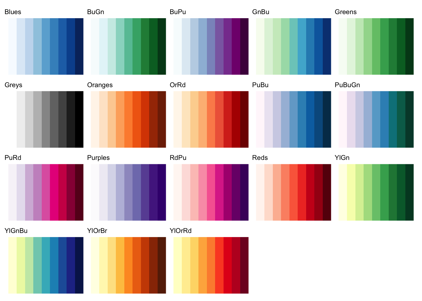
The colorNumeric() function (note the spelling of “color”) allows us to specify the colour scheme using the palette argument. The domain argument specifies the values to which that scheme will be applied. Setting an explicit domain makes sure a particular value is always assigned the same colour. The palette argument accepts the same values as the palette argument to the scale_fill_distiller() function from ggplot2:

To create the custom colour palette function, we use the <- operator to assign the result produced by colorNumeric() to a name, just as we would with an object. We can give this custom function any name we like, but in Code 9.12 we’ll call it murder_colours.

Once we have created a custom colour palette function using colorNumeric(), we can use that function to create the appropriate values for the fillColor argument of the addPolygons() function in our existing leaflet stack. Since we want the map colours to be controlled by the murder column in the district_murders object, we specify murder as the only argument to the murder_colours() palette function we have created.

Let’s see this in action: add this code to the chapter_09b.R script file:

Code 9.12

chapter_09b.R

# VISUALISE --------------------------------------------------------------------

# Create a custom colour palette function for murder counts
murder_colours <- colorNumeric(
  palette = "Reds",
  domain = pull(district_murders, "murder")
)

# Create interactive map
leaflet(district_murders) |>
  # Add base map
  addProviderTiles("OpenStreetMap.Mapnik") |>
  # Add district polygons coloured by number of murders
  addPolygons(
    fillColor = ~ murder_colours(murder),
    fillOpacity = 0.75,
    weight = 2,
    color = "black"
  )

Map 9.6

TipfillColor needs a tilde

One slight quirk of leaflet is that in order for murder_colours() to have access to the columns in the district_murders object, we need to add a tilde (~) symbol before the function name, so that the fillColor argument is fillColor = ~ murder_colours(murder) rather than fillColor = murder_colours(murder). If you forget to add the ~, you will see an error saying:

Error in murder_colours(murder) : object 'murder' not found

There are three improvements we can make to this interactive map. The first is to add a legend, using the addLegend() function. addLegend() needs three arguments:

• pal specifies which custom palette function controls the legend colours. This should be the same function as used in the fillColor argument of the addPolygons() function.
• values specifies which column in the data the legend will show. Once again, the column name should be preceded by a ~ operator.
• title specifies the legend title.

Change the code in your script file to add the addLegend() function to the end of the stack:

Code 9.13

chapter_09b.R

# Create interactive map
leaflet(district_murders) |>
  # Add base map
  addProviderTiles("OpenStreetMap.Mapnik") |>
  # Add district polygons coloured by number of murders
  addPolygons(
    fillColor = ~ murder_colours(murder),
    fillOpacity = 0.75,
    weight = 2,
    color = "black"
  ) |>
  # Add legend
  addLegend(
    pal = murder_colours,
    values = ~murder,
    title = "number of murders"
  )

Next, we can add an inset map in the corner of the main map. This is useful for interactive maps because if we zoom in to show only a small area, we will be able to use the inset map to stay aware of the wider context.

We can do this by adding the addMiniMap() function to the leaflet stack. We will add the argument toggleDisplay = TRUE to add the ability to minimise the inset map if necessary.

Update the leaflet stack in chapter_09b.R again to add the call to addMiniMap():

Code 9.14

chapter_09b.R

# Create interactive map
leaflet(district_murders) |>
  # Add base map
  addProviderTiles("OpenStreetMap.Mapnik") |>
  # Add district polygons coloured by number of murders
  addPolygons(
    fillColor = ~ murder_colours(murder),
    fillOpacity = 0.75,
    weight = 2,
    color = "black"
  ) |>
  # Add legend
  addLegend(
    pal = murder_colours,
    values = ~murder,
    title = "number of murders"
  ) |>
  # Add inset map
  addMiniMap(toggleDisplay = TRUE)

Finally, we can add labels to the districts, which will appear when we move the pointer over a district or select it on some touchscreens. We do this by adding the label argument to the existing addPolygons() function. The label will contain both the district name and murder count, so readers are not expected to estimate values from colour alone.

Change the existing call to addPolygons() to add the district labels:

Code 9.15

chapter_09b.R

# Create an interactive map of murder counts
leaflet(district_murders) |>
  # Add base map
  addProviderTiles("OpenStreetMap.Mapnik") |>
  # Add district polygons coloured by number of murders
  addPolygons(
    fillColor = ~ murder_colours(murder),
    fillOpacity = 0.75,
    label = ~ paste0(district_name, ": ", murder, " murders"),
    weight = 2,
    color = "black"
  ) |>
  # Add legend
  addLegend(
    pal = murder_colours,
    values = ~murder,
    title = "number of murders"
  ) |>
  # Add inset map
  addMiniMap(toggleDisplay = TRUE)

Map 9.7

Now we have added the extra layers to the map, we can compare districts and use the labels to read their names and values.

QuizInteractive maps

Why might a static crime map be preferred over an interactive map?

Interactive maps are illegal in some areas Static maps are easier to use in printed reports Static maps show more data Interactive maps do not allow zooming

Which of these statements is true about the relationship between the ggplot2 and leaflet packages?

Most functions from the ggplot2 package can also be used to make interactive maps with leaflet ggplot2 and leaflet are completely separate packages so none of the knowledge you might have from making ggplot2 maps can be used to make maps with leaflet The ggplot2 and leaflet packages share similar ideas (e.g. making maps using a stack of functions), but the functions in the two packages are different The leaflet package can be used to make both interactive and static maps, so the ggplot2 package is redundant

What is one advantage of interactive crime maps?

Users can zoom in and explore data dynamically Interactive maps are always more accurate than static maps Interactive maps require less data It eliminates all data errors

9.5 Calculating crime rates

The map of murders in Uttar Pradesh has a major limitation: it counts murders at district level, but it does not take into account that the number of people living in each district is different. For example, the district of Allahabad has a population of 6.0 million while the district of Mahoba has a population of 0.9 million. It’s therefore not surprising that some districts have more murders than others.

When we have crime counts for areas with populations of different sizes, it is often more useful to map crime rates instead of crime counts. A crime rate is an expression of the frequency of crime that in some way controls for the population that is exposed to crime. We often use choropleth maps for this because we typically only have population counts for areas, rather than having access to data on where each individual person lives.

9.5.1 Types of crime rate

There are three common types of crime rate, each of which measures risk in a different way. The most common, and the type of rate that people almost always mean if they talk about a ‘crime rate’ without specifying another type, is the incidence rate. This is the number of crimes in an area divided by the number of people, households or places against which a crime could occur. For example, the incidence rate of burglary in an area might be calculated as the number of crimes per 1,000 households, while the incidence rate of homicide might be expressed as the number of homicides per 100,000 people.

\[ \textrm{incidence per } k = \frac{\textrm{crimes}}{\textrm{population}} \times k \]

Here, \(k\) is the scale used to make the result easy to understand, such as 1,000 households or 100,000 residents.

Incidence rates and counts are each useful in different circumstances. For example, if you were advising a police commander on which district to allocate more homicide detectives to, the number of murders in a district is probably more useful than the incidence rate. But the opposite would be true if you were advising a politician on which district to add extra funding to for homicide prevention, since in that case you would probably want to focus on areas with the highest risk of homicide.

Important‘Incidence’ vs ‘incident’

In crime analysis, you will hear people use two very similar terms that have different meanings. When a crime analyst talks about ‘incidence’ they almost always mean ‘incidence rate’ as defined above. But when they talk about ‘incidents’ they are usually talking about the count of offences. “Which area has the most incidents?” asks about the number of offences, while “which area has the highest incidence?” asks about the rate.

Incidence rates are useful for comparing areas with each other, but they tell us a little about how likely an individual person is to be a victim of crime because crime is heavily concentrated against a few victims (think back to the law of crime concentration we discussed in Chapter 1). To understand the average risk of an individual person being a victim of crime once or more, we calculate the prevalence rate. This is the number of people, households, etc. who were victims at least once, divided by the total number of people, households, etc. in the area. Prevalence rates are usually expressed as a percentage, so we might say that 1% of the population has been a victim of a particular crime at least once during a year.

\[ \textrm{prevalence} = \frac{\textrm{victims}}{\textrm{population}} \]

The final type of rate is the concentration rate. This tells us how concentrated crime is, and is usually expressed as a single number, e.g. if the concentration rate for a crime is 2.5 then we can say that everyone who was a victim of that crime at least once was on average victimised 2.5 times. This is particularly useful for understanding how important repeat victimisation is to driving up the frequency of crime in an area. This, in turn, might lead us to focus crime-prevention efforts on work to protect recent victims of crime from being victimised again.

\[ \textrm{concentration} = \frac{\textrm{crimes}}{\textrm{victims}} \]

ImportantCrime rates are averages

All three types of crime rate are average values for an area as a whole, so we are always at risk of committing the ecological fallacy. Remember that while rates are useful for describing areas, that does not imply everyone in an area faces the same risk from crime.

9.5.2 Choosing a population measure

To calculate a crime rate, we need to be able to measure the population that is at risk from that crime. It is very common for analysts to calculate rates based on the number of people who live in an area, not least because that information is often easily available. However, there are many situations in which the residential population of an area is a poor measure of the population at risk for crime there. For example:

• Robberies in a shopping area where most of the victims do not live in the area but instead travel from elsewhere to go shopping. This can lead to vastly inflated crime rates for commercial and entertainment districts that have very small residential populations but very large numbers of people coming into the area to work, shop or visit. Crime rates based on residential population almost always give misleading rates for city centres, airports or business districts.
• Assaults on public transport where victims happen to be passing through a given area at the time they are victimised but are doing so as part of a longer journey through several areas, with the crime potentially occurring in any one of them. These crimes are known as interstitial offences.
• Residential burglaries where the targets of crime are homes, not people, so the crime rate may be influenced by the number of people in each household.

In all these cases, the residential population is a poor measure of the population at risk from crime. Unfortunately, other measures of population (such as counts of people on public transport or walking along a shopping street) are often expensive or difficult to obtain. This is known as the denominator dilemma: should we use residential population to calculate crime rates just because it is the only data that is available?

9.5.3 Calculating murder rates in Uttar Pradesh

Residential population is a conventional denominator for homicide rates and is a reasonable starting point for this example, but it is not perfect. Some victims will be killed in a different district from the one in which they live, and population counts may refer to a different year from the crime data. A detailed investigation should assess both issues before interpreting differences between districts, especially when those differences are small.

The murder counts used here are for 2014, while the population dataset contains counts from India’s 2011 census, published by the Registrar General and Census Commissioner of India. The resulting rates therefore use the closest population data available in this example, rather than the exact population in 2014. This limitation should be reported alongside the map.

To calculate an incidence rate, we once again need to join two datasets together. This time, we need to add population data for districts in Uttar Pradesh. Add this code to chapter_09b.R immediately after the code that loads the district boundaries and before the WRANGLE section:

Code 9.16

chapter_09b.R

# Download district population counts
request(
  "https://mpjashby.github.io/crimemappingdata/uttar_pradesh_population.csv"
) |>
  req_perform(path = here("data", "raw", "uttar_pradesh_population.csv"))

# Load district population counts
district_pop <- here("data", "raw", "uttar_pradesh_population.csv") |>
  read_csv(show_col_types = FALSE)

If we look at the column names in this new dataset, we will see that it includes a column called district that contains the district names. Just as we did before, we can use the left_join() function to add the columns from the district_pop dataset to the combined dataset we have already produced. To do that, let’s create a pipeline that combines all the datasets one after the other:

Code 9.17

chapter_09b.R

# Join murder counts and population to district boundaries
district_murders <- districts |>
  # Join murder counts
  left_join(murders, by = join_by(district_name == district)) |>
  # Join population counts
  left_join(district_pop, by = join_by(district_name == district))

Add this code to your script file in place of Code 9.9, which joined together the districts and murders datasets. Now look at the new district_murders object you’ve just created:

Code 9.18

R Console

head(district_murders)

Simple feature collection with 6 features and 9 fields
Geometry type: POLYGON
Dimension:     XY
Bounding box:  xmin: 77.42308 ymin: 24.80419 xmax: 82.35455 ymax: 28.90105
Geodetic CRS:  WGS 84
# A tibble: 6 × 10
  state        district_name                      geom murder code  headquarters
  <chr>        <chr>                     <POLYGON [°]>  <dbl> <chr> <chr>       
1 Uttar Prade… Agra          ((77.6444 27.23444, 77.6…    178 AG    Agra        
2 Uttar Prade… Bareilly      ((78.97474 28.41527, 78.…    132 BR    Bareilly    
3 Uttar Prade… Etah          ((79.20766 27.56734, 79.…     65 ET    Etah        
4 Uttar Prade… Shahjahanpur  ((80.30972 28.46321, 80.…     88 SJ    Shahjahanpur
5 Uttar Prade… Pilibhit      ((79.67865 28.84923, 79.…     54 PI    Pilibhit    
6 Uttar Prade… Allahabad     ((81.54684 25.1848, 81.5…    132 AH    Allahabad   
# ℹ 4 more variables: division <chr>, population <dbl>, area <dbl>,
#   density_km2 <dbl>

As with the result of the previous join, you can see that the district_murders object contains all the columns from the districts object, followed by the murder column from the murders dataset and then all the columns from the district_pop object except the district column.

Now that we have a single dataset containing all the variables we need, we can calculate the incidence of murders per 100,000 people. To do that, we can add another line of code to the end of the pipeline we have just created. Replace the existing WRANGLE section of your script file, including its section header and comments, with this code:

Code 9.19

chapter_09b.R

# WRANGLE ----------------------------------------------------------------------

# Join murder and population counts to district boundaries, then calculate the
# murder rate per 100,000 residents
district_murders <- districts |>
  # Join murder counts
  left_join(murders, by = join_by(district_name == district)) |>
  # Join population counts
  left_join(district_pop, by = join_by(district_name == district)) |>
  # Calculate murder rate
  mutate(murder_rate = murder / population * 100000)

9.5.4 Mapping crime rates

To create a choropleth map of the murder rate using leaflet, we simply use the code from our interactive map in Code 9.15 but specify that the murder_rate column be used to determine the colour of each district polygon rather than the murder column. We will also change the base map to a different style.

ImportantBe clear about how you calculated a crime rate

Whenever we map a crime rate, it is important that we are explicit about how that rate was calculated. For example, using a legend title such as “rate of murders” would not give enough information to allow readers to understand how to interpret the map. A much better legend title would be “murders per 100,000 residents” or something similar.

Whenever we need to use a longer legend title, or other text, it can be useful to break the text over multiple lines. Since leaflet maps are built using the same technologies as web pages, the way we wrap text is slightly different to how we do it when we are creating static maps. Rather than using the new-line character (\n) or the str_wrap() function, we will instead use the HTML new-line separator <br> and wrap the whole legend title in the HTML() function from the htmltools package.

Add this code to chapter_09b.R. Then read through the notes below it to understand how it differs from the map of murder counts.

Code 9.20

chapter_09b.R

# Create a colour palette for murder rates
murder_rate_colours <- colorNumeric(
  palette = "Reds",
  domain = pull(district_murders, "murder_rate")
)

# Create an interactive map of murder rates
leaflet(district_murders, elementId = "murder-rate-map") |>
  # Add base map
  addProviderTiles(
    "Esri.WorldImagery",
    options = providerTileOptions(opacity = 0.3)
  ) |>
  # Add district polygons coloured by murder rate
  addPolygons(
    fillColor = ~ murder_rate_colours(murder_rate),
    fillOpacity = 0.75,
    label = ~ paste0(
      district_name,
      ": ",
      round(murder_rate, 1),
      " murders per 100,000 residents"
    ),
    weight = 2,
    color = "black"
  ) |>
  # Add legend
  addLegend(
    pal = murder_rate_colours,
    values = ~murder_rate,
    title = htmltools::HTML("murders per<br>100,000 residents")
  ) |>
  # Add inset map
  addMiniMap(toggleDisplay = TRUE)

Map 9.8

1. This map uses a different style of base map to the previous map.
2. The base map style used in this map is quite colourful, so we will make it semi-transparent to reduce its visual prominence.
3. We want the map colour scheme to be controlled by the murder_rate column in the district_murders dataset.
4. We use the map legend title to specify how the murder rate was calculated.

We now have all the code we need to load the necessary data, calculate crime rates and make an interactive map of murders in districts in Uttar Pradesh.

9.5.5 Controlling fill colours when mapping rates

In Code 9.4 we used the code hotspot_map(car_jacking_counts) to make Map 9.4. As you can see, that the map uses colours to represent the murder rates for each district even though the code used to make the map doesn’t specify how the fill aesthetic of the data layer should be controlled (if you want to refresh your memory about map aesthetics, see Section 6.6). The code hotspot_map(car_jacking_counts) works because hotspot_map() can detect that the object car_jacking_counts was created by hotspot_count(), so hotspot_map() automatically uses the n column in car_jacking_counts to control the fill aesthetic of the data layer.

Unfortunately, automatic aesthetic selection by hotspot_map() only works when mapping objects created by other objects from the sfhotspot package (you can see another example of automatic aesthetic selection in Code 6.3). That means that when we create a dataset of crime rates by combining datasets using left_join() (as we did in Code 9.19) we have to specify which column in the data should control the fill aesthetic of the data layer on the map. We can do that using the mapping argument of hotspot_map(). For example, to make a static map of the murder rates in Uttar Pradesh districts (contained in the district_murders object we created in Code 9.19), we would use the code:

Code 9.21

R Console

hotspot_map(district_murders, mapping = aes(fill = murder_rate)) +
  labs(fill = "murders per\n100,000\nresidents")

Map 9.9

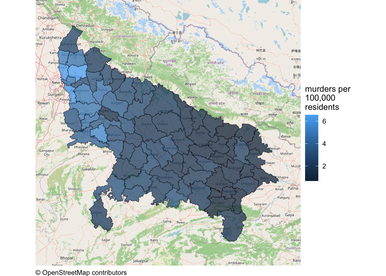
There are a couple of things to note about this map. The first is that just as we have to specify the aesthetic mapping for this map, we must also specify the legend title for the data layer using the fill argument to the labs() function.

The second notable feature of this map is that the fill scale is the wrong way around – higher murder rates are shown with lighter colours, while lower rates are shown with darker colours. As we learned in Section 7.6, when colour is used to represent data on a map, it is usually easier for readers to interpret a map if higher values are represented by darker, more-prominent colours. We also learned in Section 7.6 that we can use the scale_fill_distiller() function to control which way around the scale appears. We can add the necessary code to the stack we have already created:

Code 9.22

R Console

hotspot_map(district_murders, mapping = aes(fill = murder_rate)) +
  scale_fill_distiller(direction = 1) +
  labs(fill = "murders per\n100,000\nresidents")

Map 9.10

QuizMapping crime rates and publishing maps

What is the main difference between crime counts and crime rates?

Crime counts are more reliable than crime rates Crime counts always show higher numbers Crime rates do not tell the audience anything about the actual crime numbers Crime rates adjust for population size, while crime counts do not

What type of rate describes the chances of a person being a victim of a crime at least once in a given period?

concentration rate incidence rate incident rate prevalence rate

What type of rate describes the frequency of crime after controlling for some measure of the population at risk?

concentration rate incidence rate incident rate prevalence rate

What type of rate describes the average number of times each victim of a particular crime is victimised?

concentration rate incidence rate incident rate prevalence rate

Why is choosing the right population measure important when calculating crime rates?

To make the rates as similar as possible to crime counts, since counts are more accurate Choosing an inappropriate population measure can lead to misleading crime rates To make the crime rates as high as possible Accurate crime rates should always be the same regardless of the population measure chosen

Which action is part of publishing a crime map ethically?

Remove the legend so that the map takes up less space Publish exact victim addresses whenever they are available Explain data limitations and consider whether the map could identify or stigmatise people Assume an area-level rate applies equally to every resident

9.6 Publishing crime maps ethically

Crime maps can be used for many positive purposes. For example, they can be used to keep people safe by allowing governments to identify which areas they should focus on when trying to prevent crime by installing better street lighting or increasing police presence. Crime maps can also help citizens hold governments to account for their actions and decisions. However, as with many techniques in crime and intelligence analysis, many crime mapping techniques can also be used by totalitarian governments or other actors with malicious intent.

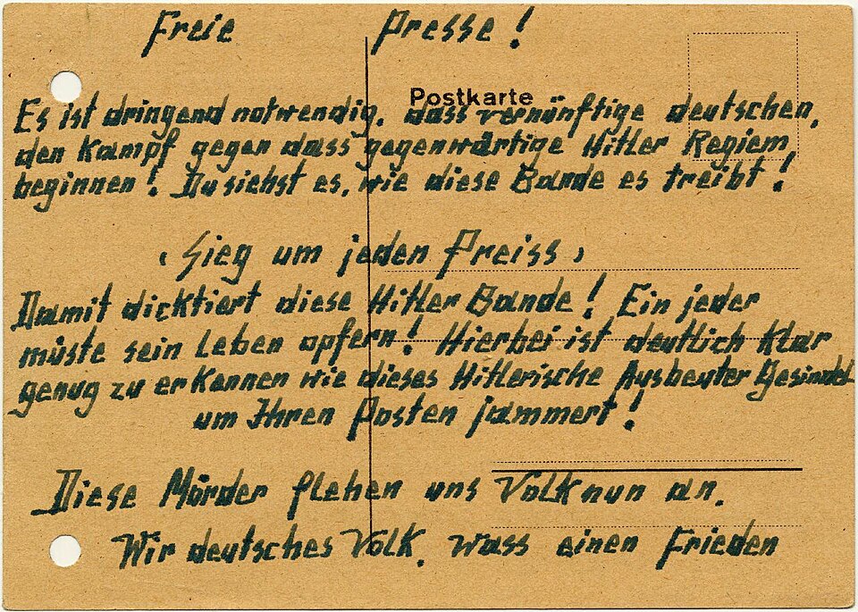
A famous example of this occurred in Germany in 1942, when the Gestapo (the Nazi secret police) used an early form of what is now called geographic profiling to identify a couple, Elise and Otto Hampel, who were distributing postcards in their neighbourhood that encouraged people to resist the Nazi regime. The Gestapo used maps of the locations where the postcards had been found to help them identify the Hampels’ home address, and they were arrested and executed.

It is always important to think of how analysis that you produce could be misused or misinterpreted, either deliberately or accidentally. This is particularly true when publishing maps of crime data, which can be used to identify victims, suspects or addresses, or to unfairly stigmatise an area and its residents.

Before sharing a map, consider:

• Privacy: could a point, label or small count allow someone to identify a victim, suspect or address? Aggregating data can reduce this risk, although very small counts may still be revealing.
• Stigma: could the title, labels or accompanying text encourage people to draw incorrect conclusions based on the ecological fallacy? For example, could people assume that a high crime rate in an area means that everyone in that area is a criminal or a victim? Could the map be used to unfairly stigmatise an area and its residents?
• Data limitations: could patterns reflect reporting or recording errors, missing locations or the choice of population measure used? State these limitations clearly.

9.7 In summary

In this chapter we practised how to calculate the number of points in different areas, join different sources of data together, and map both crime counts and crime rates using static and interactive maps. Choropleth maps can be useful, but their interpretation depends on the chosen boundaries and they only describe areas as a whole.

We have practised how to:

• count points within predefined areas using hotspot_count();
• create static and interactive choropleth maps;
• join tabular data to area boundaries and check for missing or duplicated matches;
• calculate and clearly label incidence rates;
• choose a population measure while recognising the denominator dilemma; and
• understand the ecological fallacy and modifiable areal unit problem.

Your complete chapter_09b.R script should now look like this:

Code 9.23

chapter_09b.R

# This script produces interactive maps of murder counts and murder rates in
# districts in Uttar Pradesh, India, in 2014.

# PREPARE ----------------------------------------------------------------------

# Load packages
pacman::p_load(here, httr2, leaflet, sf, tidyverse)

# Download the raw murder-count and district-boundary data
request(
  "https://mpjashby.github.io/crimemappingdata/uttar_pradesh_murders.csv"
) |>
  req_perform(path = here("data", "raw", "uttar_pradesh_murders.csv"))

request(
  "https://mpjashby.github.io/crimemappingdata/uttar_pradesh_districts.gpkg"
) |>
  req_perform(path = here("data", "raw", "uttar_pradesh_districts.gpkg"))

# Load murder counts and district boundaries
murders <- here("data", "raw", "uttar_pradesh_murders.csv") |>
  read_csv(show_col_types = FALSE)

districts <- here("data", "raw", "uttar_pradesh_districts.gpkg") |>
  read_sf()

# Download district population counts
request(
  "https://mpjashby.github.io/crimemappingdata/uttar_pradesh_population.csv"
) |>
  req_perform(path = here("data", "raw", "uttar_pradesh_population.csv"))

# Load district population counts
district_pop <- here("data", "raw", "uttar_pradesh_population.csv") |>
  read_csv(show_col_types = FALSE)

# WRANGLE ----------------------------------------------------------------------

# Join murder and population counts to district boundaries, then calculate the
# murder rate per 100,000 residents
district_murders <- districts |>
  # Join murder counts
  left_join(murders, by = join_by(district_name == district)) |>
  # Join population counts
  left_join(district_pop, by = join_by(district_name == district)) |>
  # Calculate murder rate
  mutate(murder_rate = murder / population * 100000)

# VISUALISE --------------------------------------------------------------------

# Create a custom colour palette function for murder counts
murder_colours <- colorNumeric(
  palette = "Reds",
  domain = pull(district_murders, "murder")
)

# Create an interactive map of murder counts
leaflet(district_murders) |>
  # Add base map
  addProviderTiles("OpenStreetMap.Mapnik") |>
  # Add district polygons coloured by number of murders
  addPolygons(
    fillColor = ~ murder_colours(murder),
    fillOpacity = 0.75,
    label = ~ paste0(district_name, ": ", murder, " murders"),
    weight = 2,
    color = "black"
  ) |>
  # Add legend
  addLegend(
    pal = murder_colours,
    values = ~murder,
    title = "number of murders"
  ) |>
  # Add inset map
  addMiniMap(toggleDisplay = TRUE)

# Create a colour palette for murder rates
murder_rate_colours <- colorNumeric(
  palette = "Reds",
  domain = pull(district_murders, "murder_rate")
)

# Create an interactive map of murder rates
leaflet(district_murders, elementId = "murder-rate-map") |>
  # Add base map
  addProviderTiles(
    "Esri.WorldImagery",
    options = providerTileOptions(opacity = 0.3)
  ) |>
  # Add district polygons coloured by murder rate
  addPolygons(
    fillColor = ~ murder_rate_colours(murder_rate),
    fillOpacity = 0.75,
    label = ~ paste0(
      district_name,
      ": ",
      round(murder_rate, 1),
      " murders per 100,000 residents"
    ),
    weight = 2,
    color = "black"
  ) |>
  # Add legend
  addLegend(
    pal = murder_rate_colours,
    values = ~murder_rate,
    title = htmltools::HTML("murders per<br>100,000 residents")
  ) |>
  # Add inset map
  addMiniMap(toggleDisplay = TRUE)

Save chapter_09b.R by pressing .

Check chapter_09a.R and chapter_09b.R separately, following these steps for each script:

To check that the analysis is reproducible, restart R using the Restart R (⟳) button in Positron’s Console panel, then run the script from beginning to end.

Keep the scripts in the R folder and the downloaded source files in data/raw.

To find out more about the topics covered in this chapter:

• Read the article Crime seen through a cone of resolution by Paul Brantingham, Delmar Dyreson and Patricia Brantingham for more detail about how the spatial units used in an analysis affect what we see.
• Read the article Smallest is Better? The Spatial Distribution of Arson and the Modifiable Areal Unit Problem for an example of the modifiable areal unit problem in studying crime.

QuizRevision questions

Answer these questions to check you have understood the main points covered in this chapter. Write between 50 and 100 words to answer each question.

1. If you have access to point-level crime data, why is a density map generally a better choice than a choropleth map? In what circumstances might you choose to produce a choropleth map even though you have access to the locations of individual crimes?
2. Why is the ecological fallacy a concern when interpreting crime data on choropleth maps?
3. How can crime rates provide more useful insights than simple crime counts when comparing crime levels across different areas?
4. How does choosing an appropriate population measure affect crime rate calculations?
5. Discuss the ethical considerations involved in publishing crime maps.

Hampel postcard image from Wikipedia