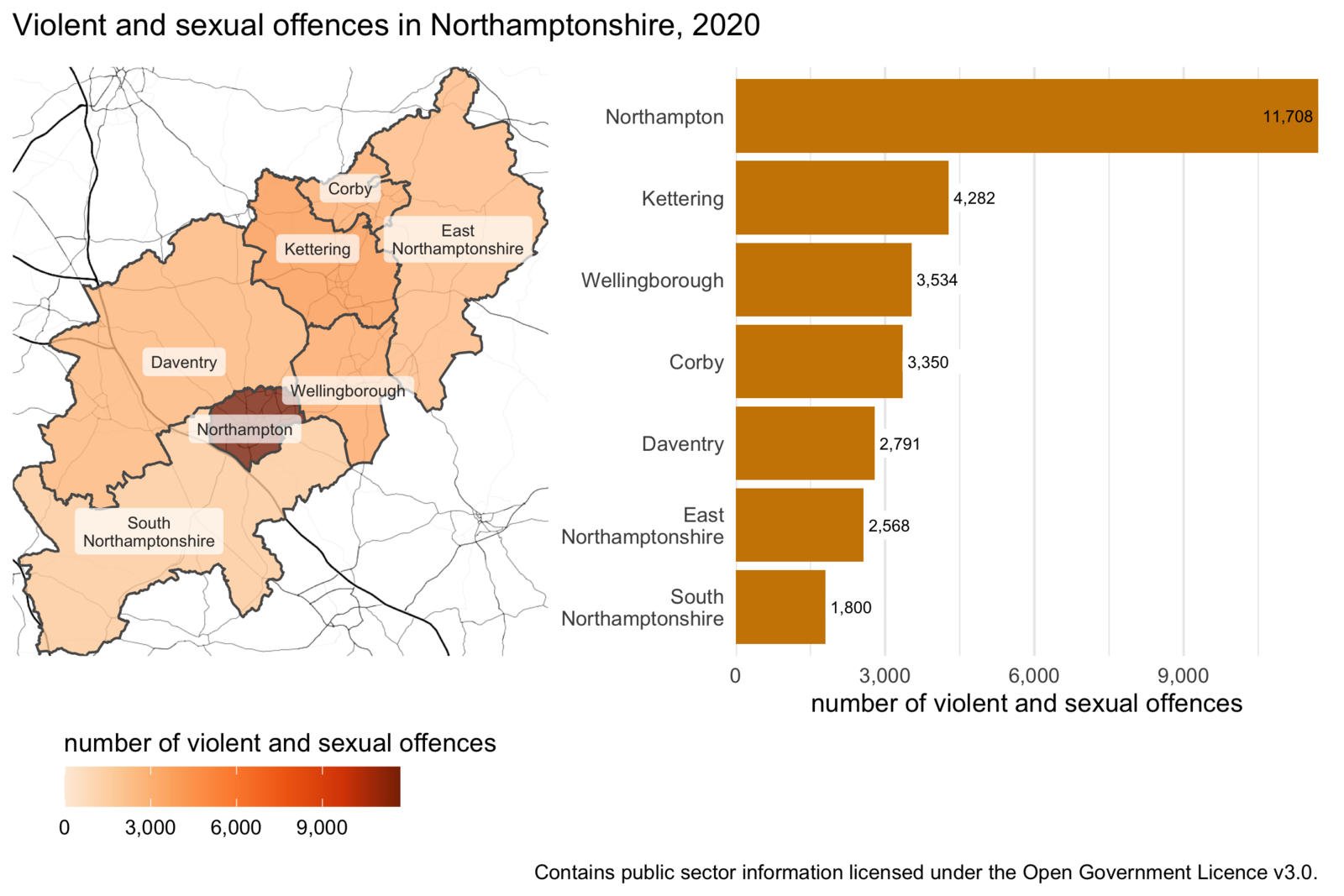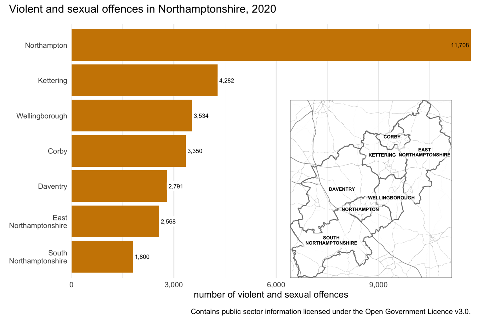
Maps are powerful tools for visualising spatial data, but they are not always the best choice. In this chapter, we will learn to choose between maps, tables and charts, then use the ggplot2 and gt packages to communicate spatial information clearly. We will create tables, bar charts, distribution plots and scatter plots, each suited to answering a different type of question.
- Open Positron or – if you already have Positron open – start a new R session by clicking the Restart R (⟳) button in the Console panel. This makes sure no code you ran previously will interfere with the work you do in this chapter.
- Make sure you are working in the crime mapping project workspace you created in Section 1.5. In the top-right corner of the Positron window, you should see a folder icon and the words
crime_mapping. If not, click the File menu, then Open Folder … and choose the crime_mapping folder.
Introduction
Making maps is the core of analysing spatial data. But just because a particular dataset has a spatial element to it does not always mean that a map is the best way to present insights from that data. In this chapter we will learn some other techniques for presenting data that can be more effective than maps for answering certain questions about spatial data.
In this chapter, we will learn how to:
- choose whether a map, table or chart is most appropriate for a particular question and audience;
- prepare data for presentation in a table;
- format a clear table using the gt package;
- use
ggauto() to create a useful first version of a chart;
- build a chart from the beginning using
ggplot();
- choose an appropriate geom for the variables you want to show;
- create and refine bar charts, raincloud plots, ridge plots and scatter plots; and
- check whether chart colours are accessible to people with different colour vision.
As with so much in spatial analysis, whether it is best to make a map or use some other technique to convey information will depend on the circumstances. When you decide how to communicate information about the data you are analysing, you will need to consider the questions you are trying to answer, the audience that you are communicating with, what they will be using the information for and in what circumstances they will be using it.
While the best choice of how to communicate spatial information will depend on the circumstances, there are a few instances in which maps are typically not the best way to communicate your data. These include:
When you need to convey several different things about one place
Maps are generally most effective when they show a single piece of data about each place (e.g. a grid cell or a polygon representing a statistical area). For example, a choropleth map shows a single shade of colour for each area on the map to represent a single value, such as the frequency or rate of crime in that area. If you wanted to show the frequency of burglary and the frequency of robbery in the same area on a map, this would be quite hard. So if you need to convey multiple different things about each place, it is generally best to do this in a table or chart, rather than a map.
One exception to this is when you present multiple maps side by side, each showing a single thing about an area. These are called small multiple maps and we will learn about them in Section 15.4.1.
When the geographic relationship between places on the map is not the most important thing about them
Maps emphasise the spatial relationship between different places, but they do this at the expense of making non-spatial relationships between those places less obvious. If the spatial relationships are the most important thing that you want to convey, a map makes sense. For example, a hotspot map is often a very good way to communicate where crime is most concentrated. But in other cases the geographic relationships between variables will be much less important. For example, if you wanted to show the relationship between the amount of crime in an area and the level of poverty there, a scatter plot would probably be a more effective way to do this than a map would be.
Tables
Well-designed tables can be a very effective way of communicating information, whereas badly designed tables can be confusing and even lead your audience to give up trying to engage with the information you’re trying to communicate.
Tables used to present information almost always show only a summary of the available data, so the first step in preparing a table is to wrangle the data into the right format. In Section 4.3 we learned about the summarise() function from the dplyr package that we can use to produce summaries of rows of data.
To learn about creating a good table for displaying summary data in a report, we will use the example of the frequency of different types of violence in the different states of Malaysia in 2017.
Create a new R script file inside the R folder of your crime_mapping workspace and save it as chapter_14a.R. Copy this code into that file and run it.
<httr2_response>
GET https://mpjashby.github.io/crimemappingdata/malaysia_violence_counts.rds
Status: 200 OK
Content-Type: application/octet-stream
Body: On disk '/Users/mattashby/Documents/Crime Mapping Book/data/raw/malaysia_violence_counts.rds' (2791 bytes)
We can get a feel for the data by looking at a random sample of rows using the slice_sample() function from the dplyr package.
# A tibble: 10 × 5
   region        state            year crime_type      count
   <chr>         <chr>           <dbl> <chr>           <dbl>
 1 West Malaysia Johor            2017 murder             66
 2 West Malaysia Kuala Lumpur     2017 armed robbery       4
 3 East Malaysia Sarawak          2017 unarmed robbery   328
 4 West Malaysia Negeri Sembilan  2017 murder             14
 5 West Malaysia Melaka           2017 murder              7
 6 East Malaysia Sarawak          2017 rape              150
 7 East Malaysia Sabah            2017 murder             36
 8 West Malaysia Pulau Pinang     2017 unarmed robbery   706
 9 West Malaysia Kuala Lumpur     2017 murder             37
10 West Malaysia Perak            2017 unarmed robbery   626
The output of slice_sample() looks acceptable as a table, especially if it is included in a Quarto document, but readers of our reports probably don’t want to know the type of each variable (underneath the variable names) and won’t want to page through the table if there are more rows or columns than can fit in the available space. We can make this table much more useful for readers by wrangling it into a different format.
Making data wider for presentation
One issue with printing the violence object as a table is that it has 70 rows, so it will take up a lot of space on a page or screen. We can make the data more compact by converting it from long format to wide format. In Chapter 10 we learned that data are often easier to analyse in long format. But it is often better to present data in a table in wide format. When you are choosing between storing data in long versus wide format, remember: analyse in long format, present in wide format.
As we learned in Chapter 10, we can convert the table to a wider format using pivot_wider() from the tidyr package. Here, the names_from argument identifies the column whose values should become new column names, while values_from identifies the column containing the values to put in those new columns.
# A tibble: 14 × 8
   region        state        year aggravated_assault armed_robbery murder  rape
   <chr>         <chr>       <dbl>              <dbl>         <dbl>  <dbl> <dbl>
 1 East Malaysia Sabah        2017                230             0     36   211
 2 East Malaysia Sarawak      2017                368             3     27   150
 3 West Malaysia Johor        2017                614             1     66   196
 4 West Malaysia Kedah        2017                364             2     21   119
 5 West Malaysia Kelantan     2017                252             2     13   114
 6 West Malaysia Kuala Lump…  2017                651             4     37   132
 7 West Malaysia Melaka       2017                176             1      7    69
 8 West Malaysia Negeri Sem…  2017                241             2     14    91
 9 West Malaysia Pahang       2017                188             1     16   163
10 West Malaysia Perak        2017                380             4     35    95
11 West Malaysia Perlis       2017                 47             0      2    30
12 West Malaysia Pulau Pina…  2017                275             0     17    80
13 West Malaysia Selangor     2017               1108            14     83   321
14 West Malaysia Terengganu   2017                130             0      5    64
# ℹ 1 more variable: unarmed_robbery <dbl>
You will be used to seeing janitor::clean_names() used to clean the column names in a dataset that has just been loaded. In this case, the new columns created by pivot_wider() will have spaces in them, because the names are taken from the values of the crime_type column in the original dataset. Column names with spaces in them a harder to work with, so this code converts them to snake case so that they are easier to work with.
Later in the code we will replace these column names with labels that are suitable for displaying the data in a table.
Now the table has only 14 rows, which makes it much easier to present both on screen and in print. We can also see that the year column is constant (all the values are the same), so we can remove this using the select() function from dplyr. We can also use select() to change the order of the columns from left to right so that the two types of robbery appear next to each other.
# A tibble: 14 × 7
   region    state murder  rape aggravated_assault armed_robbery unarmed_robbery
   <chr>     <chr>  <dbl> <dbl>              <dbl>         <dbl>           <dbl>
 1 East Mal… Sabah     36   211                230             0             284
 2 East Mal… Sara…     27   150                368             3             328
 3 West Mal… Johor     66   196                614             1            1701
 4 West Mal… Kedah     21   119                364             2             490
 5 West Mal… Kela…     13   114                252             2             219
 6 West Mal… Kual…     37   132                651             4            3175
 7 West Mal… Mela…      7    69                176             1             589
 8 West Mal… Nege…     14    91                241             2             536
 9 West Mal… Paha…     16   163                188             1             288
10 West Mal… Perak     35    95                380             4             626
11 West Mal… Perl…      2    30                 47             0              53
12 West Mal… Pula…     17    80                275             0             706
13 West Mal… Sela…     83   321               1108            14            4944
14 West Mal… Tere…      5    64                130             0             155
Using the gt package to make better tables

The table we created in Section 14.2.1 was better than simply showing the raw data to readers of a report. But we can create much better display tables with the gt package, which is designed to format data for display. The gt package works in a similar way to the ggplot2 package, in that tables are made up of stacks of functions that contribute to the appearance of the final table. One difference is that the layers in a gt stack are joined using the pipe operator (|>) rather than the plus operator (+).
We can create a very basic gt table by just passing a data frame or tibble to the gt() function. So we can add gt() to the end of the pipeline of functions we have already started to build to create a good display table. At this point, the only argument we will add to gt() is the rowname_col argument, which we use to specify which column in the data holds the row labels (in this case, the name of each state).
| Sabah |
East Malaysia |
36 |
211 |
230 |
0 |
284 |
| Sarawak |
East Malaysia |
27 |
150 |
368 |
3 |
328 |
| Johor |
West Malaysia |
66 |
196 |
614 |
1 |
1701 |
| Kedah |
West Malaysia |
21 |
119 |
364 |
2 |
490 |
| Kelantan |
West Malaysia |
13 |
114 |
252 |
2 |
219 |
| Kuala Lumpur |
West Malaysia |
37 |
132 |
651 |
4 |
3175 |
| Melaka |
West Malaysia |
7 |
69 |
176 |
1 |
589 |
| Negeri Sembilan |
West Malaysia |
14 |
91 |
241 |
2 |
536 |
| Pahang |
West Malaysia |
16 |
163 |
188 |
1 |
288 |
| Perak |
West Malaysia |
35 |
95 |
380 |
4 |
626 |
| Perlis |
West Malaysia |
2 |
30 |
47 |
0 |
53 |
| Pulau Pinang |
West Malaysia |
17 |
80 |
275 |
0 |
706 |
| Selangor |
West Malaysia |
83 |
321 |
1108 |
14 |
4944 |
| Terengganu |
West Malaysia |
5 |
64 |
130 |
0 |
155 |
This table is already better than the default table produced by Quarto if we just print a data frame or tibble. The gt table does not take up the whole width of the page unnecessarily (which can make it harder to read across rows) and has hidden the type of each column.
We can add more functions to the gt() stack to adjust the appearance of the table. For example, we can format the numeric columns as numbers using the fmt_number() function. This adds thousand separators (in British English, commas) to make it easier to read the large numeric values and can make various other changes such as adding a prefix or suffix to numbers (useful for showing units), scaling numbers (useful for very large numbers) or automatically formatting numbers according to the conventions of the language your computer is set to use (referred to in R help pages as the locale of your computer).
We choose which columns fmt_number() should format using the columns argument. In this case, we want to format all the numeric columns in the data, so we will set columns = where(is.numeric).
We don’t want the numbers in the table to have any decimal places (since the crime counts are all whole numbers), so we also set decimals = 0. We can use the default values of all the other arguments to fmt_number() – type ?gt::fmt_number in the R console to find out more about the different options available on the help page for the fmt_number() function.
| Sabah |
East Malaysia |
36 |
211 |
230 |
0 |
284 |
| Sarawak |
East Malaysia |
27 |
150 |
368 |
3 |
328 |
| Johor |
West Malaysia |
66 |
196 |
614 |
1 |
1,701 |
| Kedah |
West Malaysia |
21 |
119 |
364 |
2 |
490 |
| Kelantan |
West Malaysia |
13 |
114 |
252 |
2 |
219 |
| Kuala Lumpur |
West Malaysia |
37 |
132 |
651 |
4 |
3,175 |
| Melaka |
West Malaysia |
7 |
69 |
176 |
1 |
589 |
| Negeri Sembilan |
West Malaysia |
14 |
91 |
241 |
2 |
536 |
| Pahang |
West Malaysia |
16 |
163 |
188 |
1 |
288 |
| Perak |
West Malaysia |
35 |
95 |
380 |
4 |
626 |
| Perlis |
West Malaysia |
2 |
30 |
47 |
0 |
53 |
| Pulau Pinang |
West Malaysia |
17 |
80 |
275 |
0 |
706 |
| Selangor |
West Malaysia |
83 |
321 |
1,108 |
14 |
4,944 |
| Terengganu |
West Malaysia |
5 |
64 |
130 |
0 |
155 |
fmt_number() is one of several formatting functions available in gt. For example, we could use fmt_currency() to format columns according to the conventions for currency values, fmt_date() for dates or fmt_percent() for percentages.
The region column only has two values: West Malaysia for states and territories in Peninsular Malaysia and East Malaysia for states on the island of Borneo. Rather than repeat these two values on every row of the table – which is a waste of space and makes the table more cluttered than necessary – we can instead group the rows according to these two regions and then only show the region names once at the top of each group.
gt() will automatically create group headings in a table if the data frame or tibble passed to gt() contains groups created by the group_by() function from the dplyr package. All we have to do is use group_by() to specify which column (in this case, region) contains the values that we should use to determine which group each row is in.
| East Malaysia |
| Sabah |
36 |
211 |
230 |
0 |
284 |
| Sarawak |
27 |
150 |
368 |
3 |
328 |
| West Malaysia |
| Johor |
66 |
196 |
614 |
1 |
1,701 |
| Kedah |
21 |
119 |
364 |
2 |
490 |
| Kelantan |
13 |
114 |
252 |
2 |
219 |
| Kuala Lumpur |
37 |
132 |
651 |
4 |
3,175 |
| Melaka |
7 |
69 |
176 |
1 |
589 |
| Negeri Sembilan |
14 |
91 |
241 |
2 |
536 |
| Pahang |
16 |
163 |
188 |
1 |
288 |
| Perak |
35 |
95 |
380 |
4 |
626 |
| Perlis |
2 |
30 |
47 |
0 |
53 |
| Pulau Pinang |
17 |
80 |
275 |
0 |
706 |
| Selangor |
83 |
321 |
1,108 |
14 |
4,944 |
| Terengganu |
5 |
64 |
130 |
0 |
155 |
In tables containing lots of numbers it can be difficult to see patterns. One way to help readers to understand patterns is to map the numbers to an aesthetic property such as colour that people can easily see patterns in. To do this, we can colour the cells in a column according to the value of each cell using the data_color() function (note the spelling of ‘color’ in this function). To use data_color(), we specify the columns we want to shade using the columns argument and the colour palette we want to use using the palette argument.
In this example, we will only colour the values in two columns, so we will pass the column names to the columns argument.
The easiest way to specify a colour palette is to use one of the built-in colour palettes that the gt package understands automatically. These use the same colour palette names we have used Section 7.6 when using functions such as scale_fill_distiller().
| East Malaysia |
| Sabah |
36 |
211 |
230 |
0 |
284 |
| Sarawak |
27 |
150 |
368 |
3 |
328 |
| West Malaysia |
| Johor |
66 |
196 |
614 |
1 |
1,701 |
| Kedah |
21 |
119 |
364 |
2 |
490 |
| Kelantan |
13 |
114 |
252 |
2 |
219 |
| Kuala Lumpur |
37 |
132 |
651 |
4 |
3,175 |
| Melaka |
7 |
69 |
176 |
1 |
589 |
| Negeri Sembilan |
14 |
91 |
241 |
2 |
536 |
| Pahang |
16 |
163 |
188 |
1 |
288 |
| Perak |
35 |
95 |
380 |
4 |
626 |
| Perlis |
2 |
30 |
47 |
0 |
53 |
| Pulau Pinang |
17 |
80 |
275 |
0 |
706 |
| Selangor |
83 |
321 |
1,108 |
14 |
4,944 |
| Terengganu |
5 |
64 |
130 |
0 |
155 |
In this table we use two different colours to show the patterns in the frequency of rape and unarmed robbery. This is because we want readers to remember that different types of crime are different and so comparisons that treat crimes as being equivalent to one another are likely to be flawed. If we used the same colour across columns, readers might end up seeing that the shade used for unarmed robberies in Kuala Lumpur was darker than the shade showing the number of rapes and conclude that unarmed robberies were a bigger problem than rapes. This would be a potentially false conclusion because a single rape and a single unarmed robbery are not the same in terms of their seriousness.
For the same reason the table does not include a column showing the total number of crimes in each state – when we total all types of crime together, we are implicitly assuming that all types of crime are the same when that is obviously untrue.
Changing column names
Now that we have formatted the data, we can move onto changing the column labels. At the moment these are taken from the column names in the data, which means we have column labels such as aggravated_assault. Underscore characters (_) aren’t standard in English text, so we should change the labels to remove them. We can do this by adding the cols_label() function to the gt() stack. As well as removing the underscores, we can also use cols_label() to abbreviate labels or split them over multiple lines so that the column labels don’t force the columns to be wider than necessary.
We can use the md() helper function to use Markdown formatting to control the appearance of the labels. As well as using markup such as asterisks to create **strongly emphasised text** we can also use HTML markup to add more-advanced formatting. For example, we can use the code <br> to insert a line break to split labels over multiple lines.
| East Malaysia |
| Sabah |
36 |
211 |
230 |
0 |
284 |
| Sarawak |
27 |
150 |
368 |
3 |
328 |
| West Malaysia |
| Johor |
66 |
196 |
614 |
1 |
1,701 |
| Kedah |
21 |
119 |
364 |
2 |
490 |
| Kelantan |
13 |
114 |
252 |
2 |
219 |
| Kuala Lumpur |
37 |
132 |
651 |
4 |
3,175 |
| Melaka |
7 |
69 |
176 |
1 |
589 |
| Negeri Sembilan |
14 |
91 |
241 |
2 |
536 |
| Pahang |
16 |
163 |
188 |
1 |
288 |
| Perak |
35 |
95 |
380 |
4 |
626 |
| Perlis |
2 |
30 |
47 |
0 |
53 |
| Pulau Pinang |
17 |
80 |
275 |
0 |
706 |
| Selangor |
83 |
321 |
1,108 |
14 |
4,944 |
| Terengganu |
5 |
64 |
130 |
0 |
155 |
Adding summary rows
The final structural feature we will add is a summary row containing the total number of each type of crime across all the states and territories. We do this using the summary_rows() function from gt. We specify the columns we want to summarise using the columns argument as we did for fmt_number().
Summary rows can be produced using lots of different R functions. For example, we could use the mean() function to produce a summary row showing the mean (average) number of crimes of each type across the states. In this case, we want to know the total number of each type of crime across all states, so we will use the sum() function. To specify this, we pass the fns argument to summary_rows(). The fns argument has two parts, separated by a tilde (~). On the left-hand side we specify the label we want the summary row to have, and on the right-hand side we specify the function we want to use to calculate the summary. In this case, we can specify fns = "regional total" ~ sum(.) to say we want the summary row to have the label ‘regional total’ and that we want to summarise the rows using the sum() function. The . in the code fns = "regional total" ~ sum(.) is a placeholder that represents the data we want to summarise.
As well as summarising the data in each column, we want to specify how the summary values should be formatted. To do that, we use the fmt argument of summary_rows(). This is also a two-sided (‘formula’) argument, with the two sides separated by a ~. On the left-hand side we specify which summary values we want to format. In this case we want all the summary values to be formatted as numbers, so we can use the everything() helper function. On the right-hand side we use a call to one of the fmt_*() family of functions we used earlier: in this case, we use fmt_number(). Looking at Code 14.10, you’ll notice that the code fmt = everything() ~ fmt_number(., decimals = 0) again uses the . placeholder to specify that we want to format the summary value produced by sum().
The summary_rows() function produces a summary for each group of rows (in the case of this table, one summary for each region). As well as having a regional total, it would also be useful to have a total for all the groups together (i.e. for the whole country of Malaysia). To do that, we add the grand_summary_rows() function to our gt() stack, using the same arguments as for the summary_rows() function.
Paste this code into the chapter_14a.R file and run it.
| East Malaysia |
| Sabah |
36 |
211 |
230 |
0 |
284 |
| Sarawak |
27 |
150 |
368 |
3 |
328 |
| regional total |
63 |
361 |
598 |
3 |
612 |
| West Malaysia |
| Johor |
66 |
196 |
614 |
1 |
1,701 |
| Kedah |
21 |
119 |
364 |
2 |
490 |
| Kelantan |
13 |
114 |
252 |
2 |
219 |
| Kuala Lumpur |
37 |
132 |
651 |
4 |
3,175 |
| Melaka |
7 |
69 |
176 |
1 |
589 |
| Negeri Sembilan |
14 |
91 |
241 |
2 |
536 |
| Pahang |
16 |
163 |
188 |
1 |
288 |
| Perak |
35 |
95 |
380 |
4 |
626 |
| Perlis |
2 |
30 |
47 |
0 |
53 |
| Pulau Pinang |
17 |
80 |
275 |
0 |
706 |
| Selangor |
83 |
321 |
1,108 |
14 |
4,944 |
| Terengganu |
5 |
64 |
130 |
0 |
155 |
| regional total |
316 |
1,474 |
4,426 |
31 |
13,482 |
| national total |
379 |
1,835 |
5,024 |
34 |
14,094 |
Save chapter_14a.R by pressing . Your complete table script should now look like this:
To check that the analysis is reproducible, restart R using the Restart R (⟳) button in Positron’s Console panel, then run the script from beginning to end.
Tables are good for showing detailed information, particularly when we want to present multiple pieces of information about a single place. But it can be hard to spot patterns in tables even with coloured cells. For this reason, do not use tables when you are primarily trying to show the relationship between two or more variables. In Section 14.3, we will learn to create a bar chart in R to show patterns more effectively.
Making charts with ggplot2 and ggauto
In Section 6.6 and Chapter 7, we created maps with hotspot_map() and refined them with functions from the ggplot2 package. Behind the scenes, hotspot_map() constructs a map using other functions from the ggplot2 package, by default making choices that try to produce a good map. We can’t use hotspot_map() to make these choices for us when we are creating charts because it is specialised for creating maps. Instead, we can use the ggauto() function (from the package of the same name) to automatically choose a type of chart that is likely to be appropriate for the data we are working with. We can then use functions from the ggplot2 package to refine the chart in the same way we have refined maps.
ggauto() can create several different types of chart automatically. It chooses which type of chart to make based on how many variables we want to visualise and whether the variables are continuous (e.g. numbers), dates/times (which we will learn more about in Chapter 15), ordered categories or unordered categories. There are some types of chart that ggauto() can’t handle, or for which the chart produced by ggauto() might not be appropriate for particular audiences. In those cases, we can use functions from the ggplot2 package to create a chart from scratch and then refine it to suit our needs.
To see how this works, let’s start by creating a bar chart. Bar charts are useful for showing values of one numeric variable (e.g. a count of crimes) for each value of one categorical variable (e.g. states of a country). Before we create a bar chart, create a new R script file in the R folder of your crime_mapping workspace and save it as chapter_14b.R. Copy this code into that file and run it.
<httr2_response>
GET https://mpjashby.github.io/crimemappingdata/malaysia_violence_counts.rds
Status: 200 OK
Content-Type: application/octet-stream
Body: On disk '/Users/mattashby/Documents/Crime Mapping Book/data/raw/malaysia_violence_counts.rds' (2791 bytes)
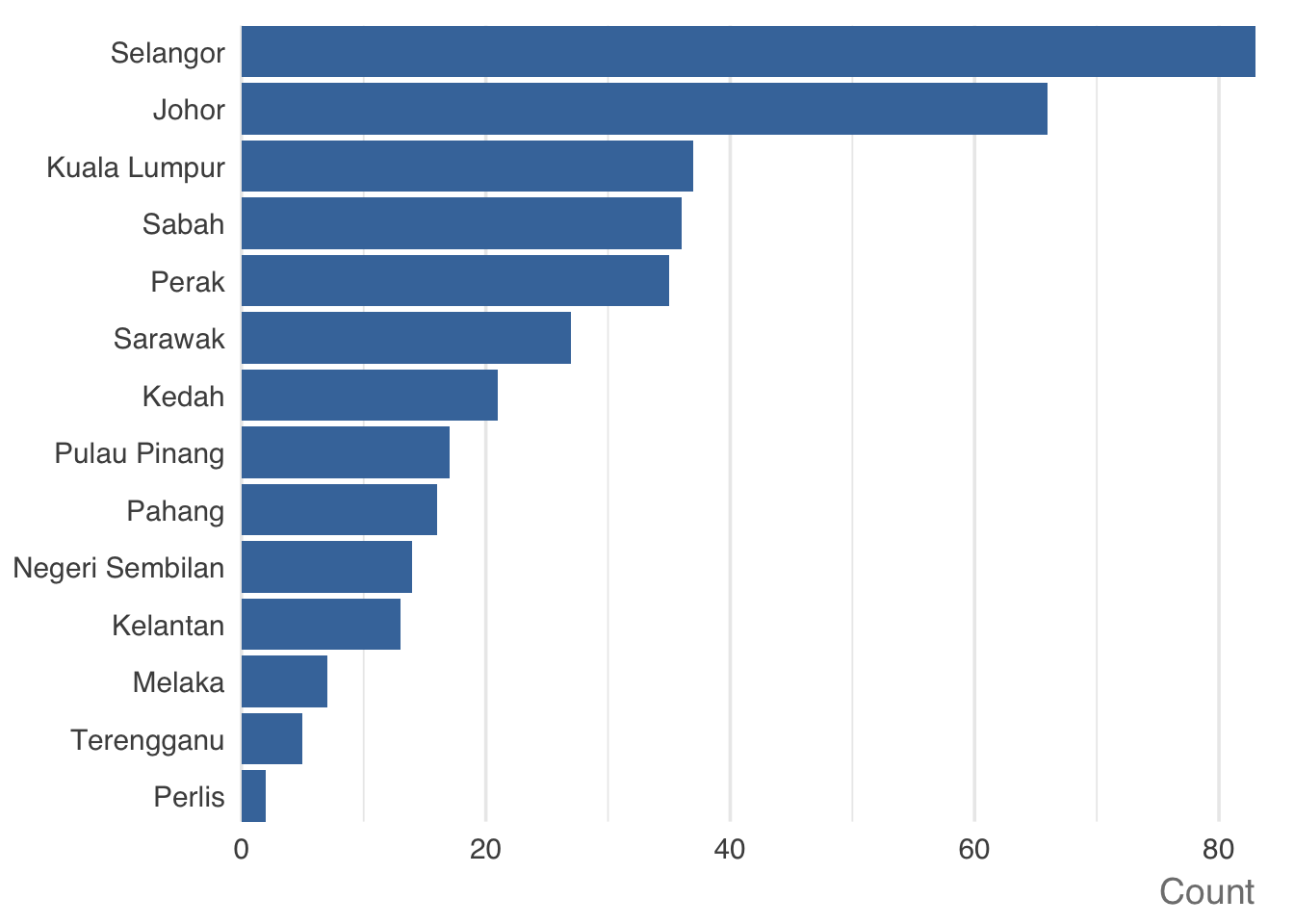
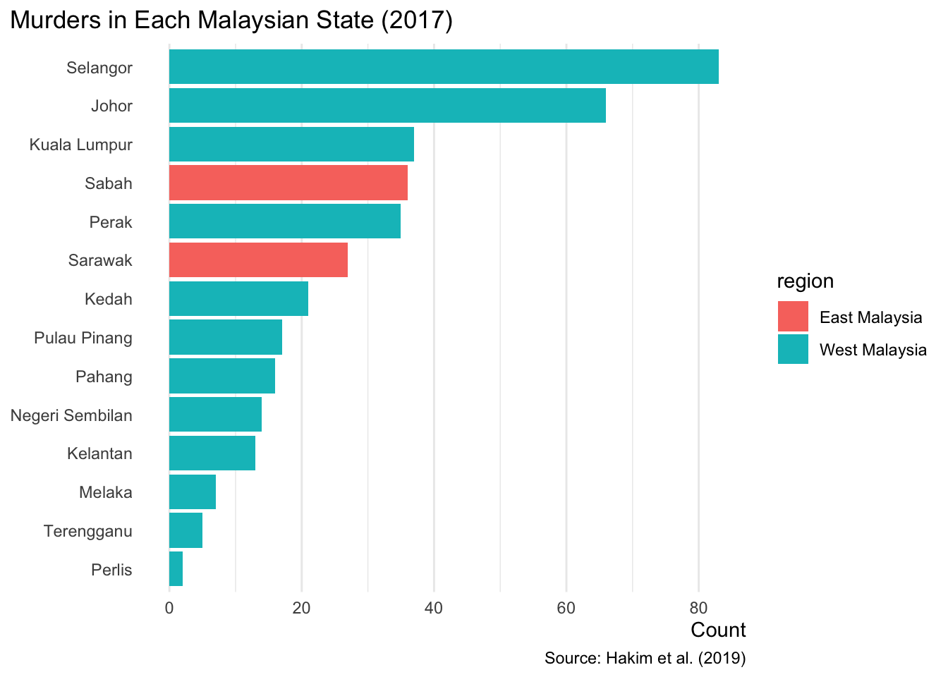
By default, ggauto() produces a useful starting point for a bar chart, so let’s use it to show the number of murders in each Malaysian state in 2017. We will use the violence object we created earlier, which contains counts of different types of violence in each state.
The :: notation tells R to use the ggauto() function from the ggauto package without first loading the whole package. We only use ggauto interactively in the R Console in this chapter, rather than using it in the scripts we are building, so there is no need to load it at the start of those scripts. The ggauto package must still be installed on your computer for this code to work.
There are several features of the bar chart created by ggauto() that make the chart easier for readers to use than many bar charts produced by default in other software. Specifically:
- The bars are horizontal, not vertical. This means that the state labels can also be horizontal, which is very useful because in English we read text horizontally and so it’s easier to read horizontal text than vertical text. Horizontal bar charts are almost always better than vertical ones when we need to show non-numeric category labels.
- A lot of clutter that is sometimes included in default charts has been removed if it isn’t needed for this particular type of chart. For example, there are no tick marks between the bars and the state names.
- The chart includes a title for the horizontal axis (known as the x-axis) so that readers know what the numbers represent, but there is no title for the vertical axis (known as the y-axis) because it is obvious from the context that the vertical axis shows the names of the states.
- The states have been ordered so that the states with the most murders have been shown at the top of the chart and the states with the fewest murders have been shown at the bottom. This makes it easy for readers to see which states have the most and fewest murders. Ordering the bars like this is almost always better than using the default alphabetical order of the state names.
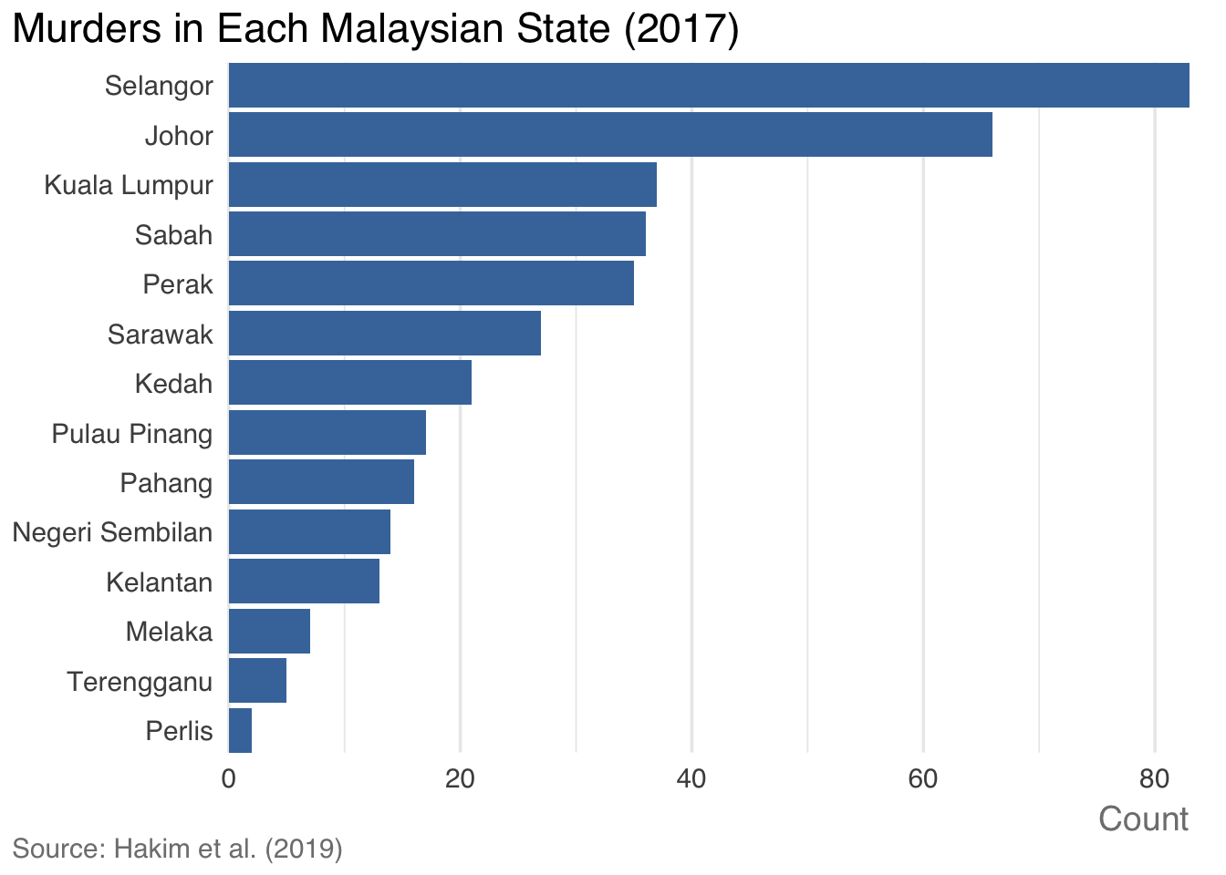
The chart produced by ggauto() is a useful starting point, but we can make it more informative by adding a title and caption. We can do this using the labs() function from the ggplot2 package that we learned about in Section 7.8. Let’s add a title showing what the chart shows and a caption giving the source of the data. In this case, the data comes from an academic paper written by Hashom Hakim and colleagues.
Note that because ggauto() produces a chart, we need to add subsequent functions such as labs() with the + operator rather than the |> operator.
ggauto() has produced a useful bar chart, but to go any further we need to learn to construct charts ourselves using the full range of functions from the ggplot2 package. For example, we might need to do this if we wanted to change the colour of the bars so that the bar for each state was coloured according to which region it was in.
We can start to learn how to create charts from scratch using functions from ggplot2 by looking at the code that would be needed to reproduce the bar chart in Figure 14.4 without using ggauto(). Look through Code 14.15 and its accompanying explanations.
- 1
-
In order for the bars to be displayed in descending order of the number of murders, we need to reorder the
state column in the data. To do this we convert that column to something R calls a factor, which is capable of storing a meaningful order for the categories. We will learn more about this in Section 14.3.1.
- 2
-
The
ggplot() function takes a dataset and initiates a new chart. However, ggplot() (unlike ggauto()) doesn’t produce a chart on its own. We need to add more components to the chart before it can be displayed. You can think of ggplot() as telling R “I want to make a chart using this data”.
- 3
-
The
aes() function specifies which columns in the data will control which aesthetics of the chart. We learned about aesthetics in Section 5.6.1 and about the aes() function in Section 6.6. In this case, we want the count column to control the horizontal position of the end of each bar and the state column to control the vertical order of the bars.
- 4
-
The
geom_col() function tells R that the chart we want to create should be a bar chart. While ggplot() says “I want to make a chart using this data”, geom_col() says “the chart should be a bar chart”. The argument fill = "#4477AA" specifies what colour we want the bars to be.
- 5
-
The
labs() function adds titles and captions to the chart, as we learned in Section 7.8. We can also use labs() to control the titles of the axes on the chart. In this case, we set y = NULL to remove the title for the vertical axis, since a title is unnecessary when it is obvious from the context what the values on that axis represent (Malaysian states).
- 6
-
The
theme_minimal() function controls which ggplot2 theme the chart uses. Themes control the supporting elements of a visualisation, such as the appearance of grid lines, which font is used for text, etc. We will learn more about themes in Section 14.3.2.
- 7
-
The
theme() function allows us to make further refinements to the theme used by the chart. There are lots of ways we can customise a chart theme. In this case we’ve removed the default horizontal grid lines (which aren’t useful for horizontal bar charts), made the x-axis title right-aligned and moved the chart title to the top-left corner of the chart.
Now you’ve seen how much code is needed to create a bar chart from scratch, you can see why ggauto() is useful for quickly producing a sensible starting point. However, sometimes we will need to go beyond what ggauto() can do, so it’s useful to know how to create charts from scratch. Before we go beyond what ggauto() can do for us, we will first delve a bit deeper into some aspects of Code 14.15 that we haven’t already covered.
Controlling the order of categorical variables
If you were trying to find the three Malaysian states or territories with the most murders from this chart, it would be pretty easy to see on any bar chart that Selangor had the most murders, followed by Johor. But at a glance, it might not so easy to see which state or territory comes third unless the bars are ordered by their values. This is why alphabetical ordering of bars (which is the default used by ggplot2) is almost never the best choice for a bar chart.
To order the bars according to the number of murders in each state, we need to convert the state column in the data to a new type of variable: a factor. Factors are what R calls categorical variables that have (a) a defined set of possible values and optionally (b) a defined order of values.
One of the benefits of storing a variable as a factor is that we can specify an order for the categories. This is useful for categories that have a meaningful order, such as ‘bad’, ‘acceptable’, ‘good’, ‘excellent’. But we can also use this feature of factors to specify that values should appear in a particular order in any charts produced from the data, whatever the order of the values in the data itself.

To work with factors in R we can use the forcats package, so-called because it’s for working with categories. forcats is loaded as part of tidyverse, so we don’t need to load it separately.
All the functions in the forcats package start with the letters fct_, just as all the functions in the sfhotspot package start hotspot_. For our bar chart, we will use the fct_reorder() function. This takes a factor or character variable (such as the names of the Malaysian states and territories) and sets the order of the categories according to the values of a numeric variable (such as the number of murders in a state). So to re-order the state variable according to the count of murders, we can use fct_reorder(state, count). Since we’re changing an existing variable, we do this inside a call to the mutate() function that we learned about in Section 4.2. Look back to the code in Code 14.15 and you will see the line mutate(state = fct_reorder(state, count)).
ggplot2 themes
The theme_*() family of functions in ggplot2 allows us to control all the non-data elements of a chart. These are the elements that support the data shown by the geoms (e.g. bars, points, lines) in a chart, such as the background, grid lines, axis text and the appearance of titles and legends. It’s important to note the distinction about what we can control with themes and what we cannot. Themes control the supporting elements of a visualisation rather than the data shown by its geoms. Changing the theme will not change anything about how the data is represented in a chart, such as the colour of bars.
There are many different themes that you can add to a ggplot() stack. Some of these are built into the ggplot2 package, and some are part of other packages that extend what ggplot2 can do. Some organisations (such as the BBC) have their own ggplot2 themes for creating maps and charts that follow their corporate style guide.
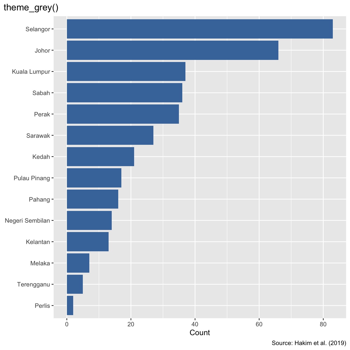
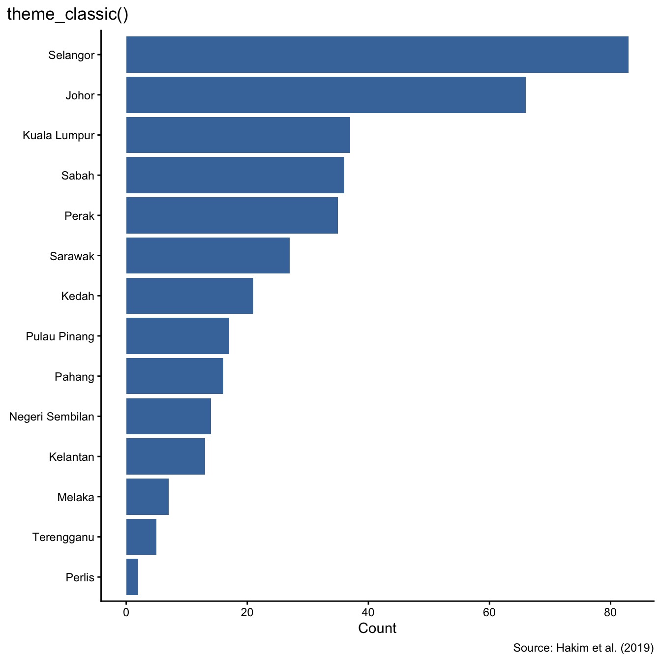
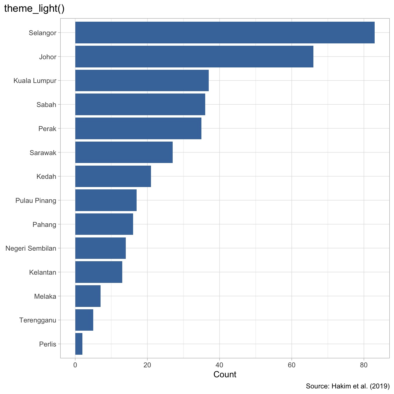
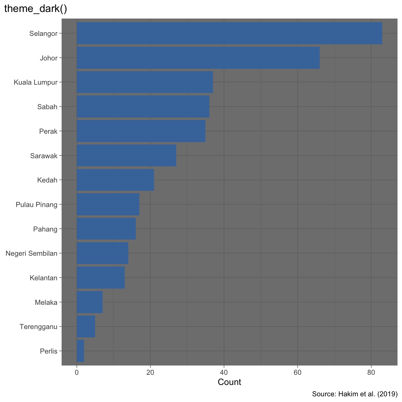
Different themes can give charts very different appearances, even when they use the same data. For example, these four charts show what happens when different themes are applied to the end of the same ggplot() stack:
If we don’t specify a theme, ggplot2 will use the default theme, which is called theme_grey(). This theme is useful for exploring data because it includes grid lines and other elements that make it easier to see the values of the data. But when we are creating a chart for an audience, we usually want to remove unnecessary elements that don’t communicate useful information. It’s important to remove any unnecessary elements from our charts to help the audience focus on the most-important elements. For that reason, we will usually use theme_minimal() for charts, which removes the background colour and panel border while retaining grid lines that can help readers estimate values. If you look back at the code in Code 14.15 you can see that it uses theme_minimal() and then removes the horizontal grid lines that are not useful for this chart.
One of the theme_*() family of functions can go a long way to improving the appearance of a chart, but we will sometimes also need to make further adjustments to make sure the chart is as clear as possible. We can do this using the theme() function, which allows us to make further refinements to the theme used by the chart.
There are many different elements of a chart that we can control using the theme() function. For example, we can control the appearance of the chart title, the axis titles, the axis text, the legend and the background. In Code 14.15 we used several arguments of the theme() function.
- We set
axis.title.x to element_text(hjust = 1) to right-align the title of the horizontal axis. element_text() is one of a family of helper functions that ggplot2 provides so that we can easily control the appearance of different elements within a theme. As the name suggests, element_text() is the function within this family that we can use to control the appearance of non-data text on the chart, such as the chart title, axis labels, etc. The hjust argument controls the horizontal alignment of text, with a value of 0 meaning left-aligned, a value of 1 meaning right-aligned and a value of 0.5 (the default) meaning centred.
- We set
panel.grid.major.y and panel.grid.minor.y to element_blank() to remove the horizontal grid lines that run along the length of the bars, since they don’t really make it any easier to understand the chart. element_blank() is a helper function that sets the specified element to be blank.
- We set
plot.title.position = "plot" to specify that we want the chart title to appear in the top-left corner of the whole chart rather than being aligned only with the edge of the plotting area. We almost always want the chart title to appear in this way, so we will use this code often.
Colour in bar charts
Now that we have successfully used ggplot() to recreate the bar chart created by ggauto(), and understood all the code needed to do that, we can go on to further improve the chart by adding colour to the bars to indicate which region of Malaysia each state is in.
To do that, we need to add another mapping to the aes() function that is included in Code 14.15 and which controls which columns in the violence dataset control which elements of the chart. aes() already specifies that the count column controls the horizontal position of the end of each bar and that the state column controls the vertical order of the bars. We can add another mapping to aes() to specify that the fill colour of the bars should be controlled by the region column in the data. This will colour each bar according to which region of Malaysia it is in. Run this code in the R console to see the result. Note that this time we are saving the result in an object called malaysia_murder_bar_chart so that we can use the result again shortly.
As well as changing aes(x = count, y = state) to aes(x = count, y = state, fill = region) there is one other difference between the Code 14.16 and Code 14.15: we have changed geom_col(fill = "#4477AA") to geom_col(). If we had not done that, specifying which column in the data should control the fill aesthetic would have had no effect, since static aesthetics specified in geom_col() override the same aesthetic specified inside aes(). If you ever specify the colour or fill aesthetics inside aes() and it doesn’t seem to have any effect, check that you haven’t also specified a constant value for the same aesthetic inside the geom_*() function.
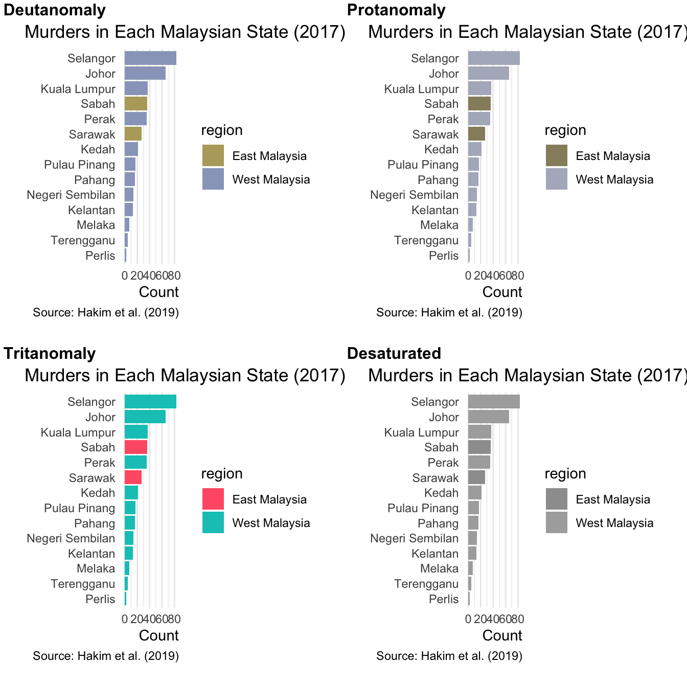
One issue with this chart is that the default colours that ggplot() produces are not easy for everyone to discern. In particular, people with colour blindness may struggle to distinguish between some combinations of colours. Some colour combinations are also hard (or impossible) to distinguish even for people with normal colour vision if a chart is printed in black and white or viewed on a screen in some lighting conditions.
We can check how well people with different colour vision will be able to read a chart using the cvd_grid() function from the colorblindr package. This function takes an existing ggplot() stack and prints several versions of the chart that simulate how different people will see it.
The colorblindr package is not on CRAN, the repository we usually install R packages from. That means we need to use slightly different code to install it. Instead of installing from CRAN, we will instead install the package from GitHub, a website that programmers use to store versions of their code. To install packages from GitHub we can use the p_install_gh() function from the pacman package (the same package we use to load packages at the start of each R script).
Remember that because we only need to install a package once on each computer we use R on, you should never install packages inside an R script. This means you should only ever run pacman::p_install_gh() in the R Console, never in an R script.
Once you’ve installed the colorblindr package, you can use it to check how different people are likely to see the chart of murders in Malaysia.
From this we can see that this combination of colours works well for people with some types of colour blindness, but is likely to be hard for some people, and indeed for everyone if the chart is printed on a black-and-white printer.

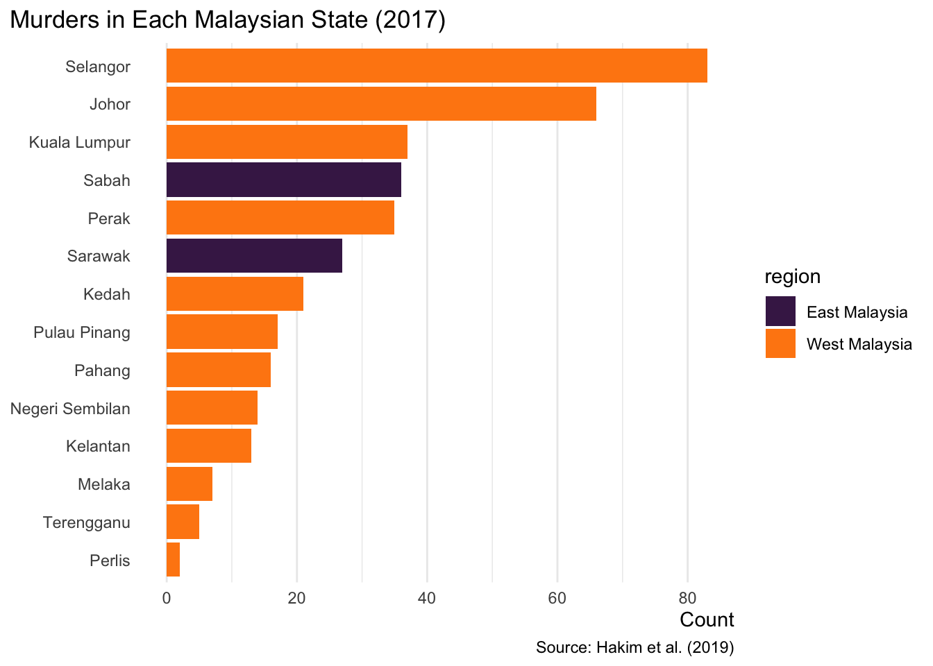
Fortunately, there are lots of different R packages that provide colour palettes that are suitable for people with different colour vision. The paletteer package brings a lot of these colour palettes together in one place. paletteer provides three pairs of functions for different types of colour scale:
scale_colour_paletteer_c()/scale_fill_paletteer_c() for continuous scales that are suitable for representing continuous variables.scale_colour_paletteer_d()/scale_fill_paletteer_d() for discrete scales that are suitable for representing categorical variables.scale_colour_paletteer_binned()/scale_fill_paletteer_binned() for binned scales that are suitable for showing continuous variables that have been sub-divided (‘binned’) into ordered categories.
We can use each of these functions in the same way we have used functions like scale_fill_distiller() in Section 7.6. The first argument to all the main functions in the paletteer package is the name of a colour palette, of which a total of 2,893 different palettes are available. We can specify which palette to use using the same syntax we have sometimes used to refer to R functions: package_name::palette_name. For example, to create a discrete colour scale using the OKeeffe2 palette from the MetBrewer package (a palette inspired by the painting Red and Yellow Cliffs by Georgia O’Keeffe) we could use scale_colour_paletteer_d("MetBrewer::OKeeffe2").
There are many useful colour palettes in the PrettyCols package. Let’s use the Bright palette from this package to control the colours on the chart. This is the final version of the code needed to make the bar chart we want, so we will save it in the chapter_14b.R file and then run it to see the finished result.
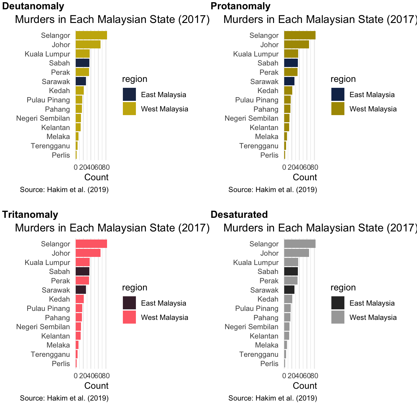
To see if these colours are likely to work for different people, we can again check the colours with the colorblindr package:
From this, we can see that this colour palette is going to be much more useful for people with different colour vision, as well as for everyone if the chart is printed in black and white or viewed on a screen in bad light.
Bar charts are a very common way of presenting a numeric variable for each value of a categorical variable. Bar charts are easy to interpret, even for people who are not used to interpreting charts or who only have time to look at the chart for a few seconds.
Save chapter_14b.R by pressing . Your complete bar-chart script should now look like this:
To check that the analysis is reproducible, restart R using the Restart R (⟳) button in Positron’s Console panel, then run the script from beginning to end.
If the code does not run successfully, that might mean you have forgotten to include some of the code that is needed to make the chart.
Visualising distributions
Bar charts show a single piece of information about each category present in a dataset. So we might use a bar chart to show, for example, the average number of burglaries in neighbourhoods in different districts. But what if the average values masked substantial differences in the number of burglaries within each district? Averages often mask variation, and can sometimes be misleading as a result. In those circumstances it would be better to show more detail rather than a misleading average.
Let’s start with the simple example of showing the distribution of burglary counts within the English county of Northamptonshire. Start a new R session by clicking the Restart R (⟳) button in Positron’s Console panel. Create a new R script inside the R folder and save it as chapter_14c.R. Use this code to download and load a dataset of burglaries in each lower-layer super output area (LSOA) in Northamptonshire in England in 2020. LSOAs are small geographic areas that are used for many statistical purposes in England. Each LSOA covers about 1,500 households.
<httr2_response>
GET https://mpjashby.github.io/crimemappingdata/northants_burglary_counts.rds
Status: 200 OK
Content-Type: application/octet-stream
Body: On disk '/Users/mattashby/Documents/Crime Mapping Book/data/raw/northants_burglary_counts.rds' (1953 bytes)
So that we can see what this dataset looks like, we first run head() in the R Console:
# A tibble: 6 × 3
  district lsoa       count
  <chr>    <chr>      <int>
1 Corby    Corby 001A     6
2 Corby    Corby 001B     7
3 Corby    Corby 001C     5
4 Corby    Corby 001D    29
5 Corby    Corby 002A     9
6 Corby    Corby 002B     3
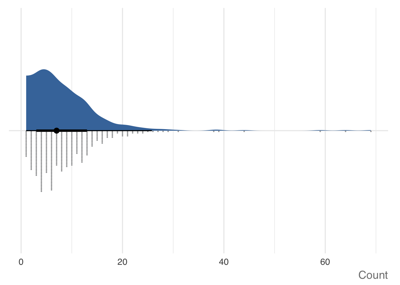
We can start the process of producing a chart by seeing what type of chart ggauto() produces when we give it a continuous (numeric) variable rather than (as in Figure 14.3) a categorical variable. Run this code in the R console to see the result.
This type of chart is called a raincloud plot, because it looks like rain falling from a cloud. It shows us the distribution of the data in three ways:
- At the top is a density plot showing us the overall distribution of the count of burglaries in LSOAs in Northamptonshire.
- In the middle is a black bar, which shows the inter-quartile range of the data: the range of values that contains the middle 50% of the data. The ends of the black bar show the first and third quartiles, which are the values that divide the lowest 25% and highest 25% of the data from the middle 50%. The black dot in the middle of the black bar shows the median value, which is the value that divides the lower half of the data from the upper half.
- At the bottom is a plot in which each LSOA is shown as a dot and the dots are stacked according to how many burglaries occurred in that LSOA.
All three of these elements show the same information, but in different ways. We can, for example, see that most LSOAs had only a few burglaries in 2020, while a small number of LSOAs had substantially more. This is what we would expect, since we learned in Section 1.3 that crime is heavily concentrated in a few places.
Raincloud plots can be very useful, but really only if your audience is already familiar with interpreting them. Many audiences for crime analysis, such as police leaders or community representatives, may not be familiar with raincloud plots and so might find them confusing or off-putting. A simpler way of showing the distribution of a numeric variable is a ridge plot, which shows only the density plot from a raincloud plot.
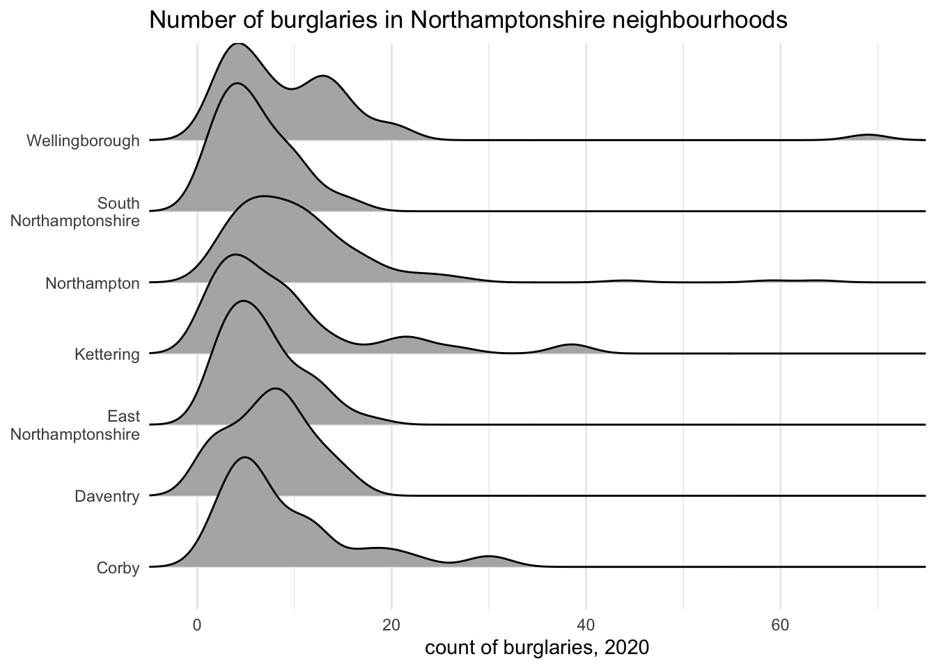
We can create a ridge plot with the geom_density_ridges() function from the ggridges package. This function does not come from the ggplot2 package, but is designed to be used inside a ggplot() stack. Ridge plots are particularly useful for showing the distribution of a numeric variable across multiple categories at once. For example, we could show the distribution of burglary counts at the neighbourhood level for all the districts in Northamptonshire.
Add this code to the chapter_14c.R file and run it.
Picking joint bandwidth of 1.98
As we explored in Section 6.2.2, density estimation depends on us choosing a bandwidth to control the degree of smoothing between data points. By default, geom_density_ridges() chooses a suitable bandwidth automatically and reports this in a message. The bandwidth is referred to as ‘joint’ because the same bandwidth is used for all the density curves on a chart.
If you wanted to include a ridge plot in a Quarto document, you would probably not want this message to appear in your report. To suppress the message, you can use the Quarto chunk option #| message: false.
The ridge plot shows the distribution of burglary counts in LSOAs within each district, with the distributions overlapping slightly to save space. From this we can see that across all districts most LSOAs have few burglaries, with a small number of LSOAs having more. We can also see (top-right of the chart) there are a small number of LSOAs (probably, in fact, just one LSOA) in Wellingborough district with a much higher number of burglaries than anywhere else in Northamptonshire.
Save chapter_14c.R by pressing . Your complete distribution-analysis script should now look like this:
To check that the analysis is reproducible, restart R using the Restart R (⟳) button in Positron’s Console panel, then run the script from beginning to end.
Comparing continuous variables
So far we have used bar charts to communicate a single number (in our example, a number of murders) for each value of a categorical variable (the name of each Malaysian state or territory), and ridge plots to show multiple numbers (burglary counts for each neighbourhood) for each value of a categorical variable (districts in Northamptonshire).
Both these types of chart compare a numeric variable to a categorical one. But sometimes we may want to compare two numeric variables. We can do this with a scatter plot.
Start a new R session by clicking the Restart R (⟳) button in Positron’s Console panel. Create a new R script inside the R folder and save it as chapter_14d.R. Use this code to download and load rates of thefts of and from motor vehicles per 1,000 households saying they own a vehicle for a selection of municipalities in South Africa.
<httr2_response>
GET https://mpjashby.github.io/crimemappingdata/south_africa_vehicle_theft.rds
Status: 200 OK
Content-Type: application/octet-stream
Body: On disk '/Users/mattashby/Documents/Crime Mapping Book/data/raw/south_africa_vehicle_theft.rds' (5387 bytes)
Let’s look at the dataset in the R Console in the usual way:
# A tibble: 6 × 4
  province     municipality     crime_category                     theft_rate
  <chr>        <chr>            <chr>                                   <dbl>
1 Eastern Cape Amahlathi        Theft of motor vehicle                   2.49
2 Eastern Cape Amahlathi        Theft out of or from motor vehicle      26.4
3 Eastern Cape Blue Crane Route Theft of motor vehicle                   6.05
4 Eastern Cape Blue Crane Route Theft out of or from motor vehicle      19.1
5 Eastern Cape Buffalo City     Theft of motor vehicle                   7.58
6 Eastern Cape Buffalo City     Theft out of or from motor vehicle      49.0
Since thefts of vehicles and thefts from vehicles are different but related crimes, we might want to see if there is a relationship between the rates of each type. We can do that using a scatter plot.
The data in the vehicle_theft object are in long format, with each row representing a crime rate in a particular category for a particular municipality. To make a scatter plot where each point represents a municipality, we need to have all the data for a municipality in a single row of data, so we will transform the data with pivot_wider() (as we did for some of the tables at the start of this chapter). This converts the values of the crime_category column into column names. These names are quite long, so we first convert them to snake case using janitor::clean_names() and then use rename() to shorten the names so they are easier to work with.
Replace the code in chapter_14d.R that loads the data with this code.
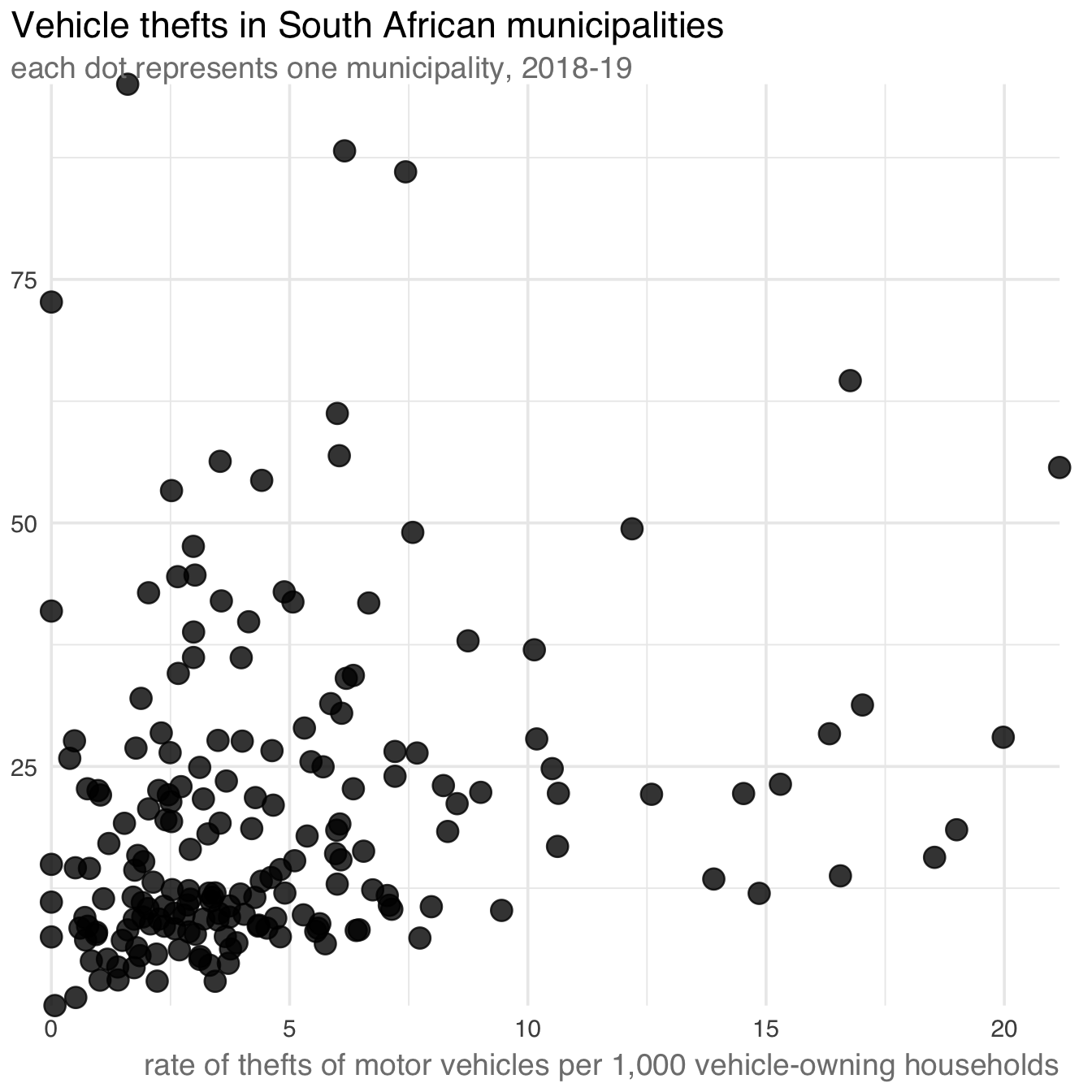
We can now use ggauto() to make a basic scatter plot.
This chart generally looks good, but you might be able to spot a problem: the y-axis is not labelled correctly. In the background, ggauto() tries to use a trick to make the y-axis label appear horizontally, so it is easier to read. Unfortunately that trick doesn’t work when we specify a subtitle for the plot, or when we try to specify the y-axis title with labs(). Fortunately, the code needed to replicate this chart with ggplot() is quite simple, so in this example we don’t add much more complexity by not using ggauto().
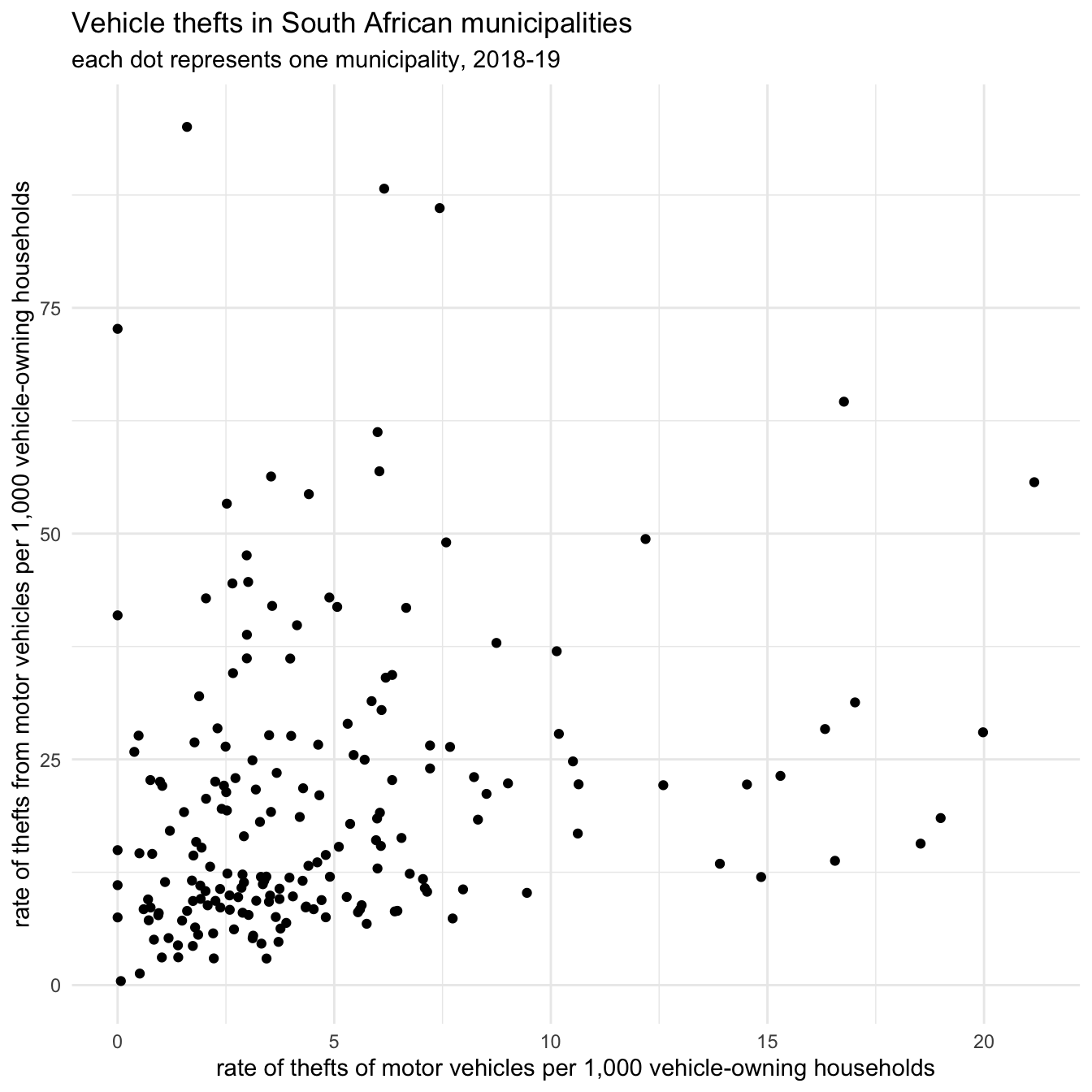
Run this code in the R Console.
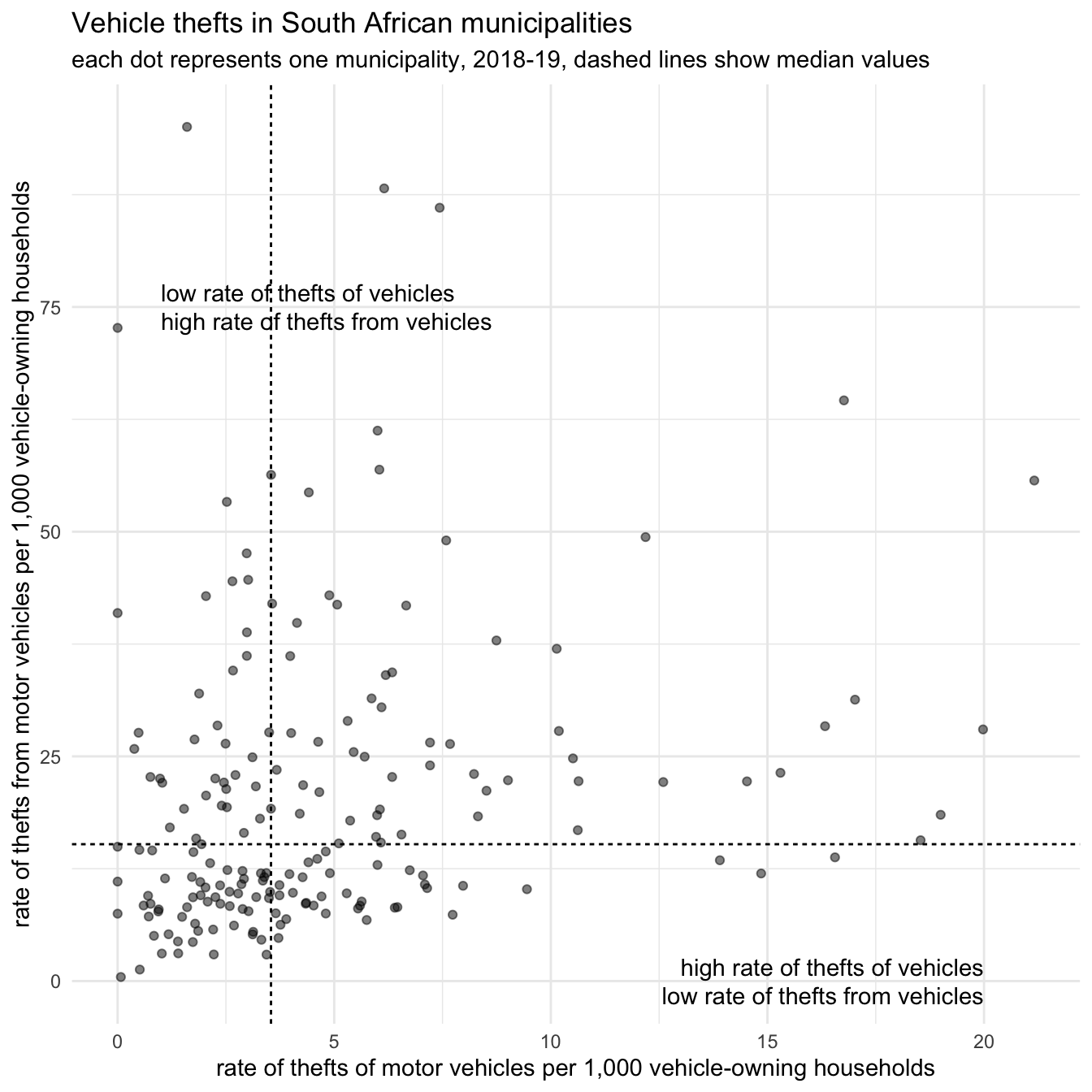
From this plot we can see that most areas have low rates of both theft of and theft from motor vehicles, with a few areas having very high rates of one type or the other (but none have high rates of both).
Looking at the bottom-left corner of the chart we can see that we have again encountered the problem of overlapping points making patterns less clear. We can try to deal with this by making the points semi-transparent using the alpha argument to geom_point().
Scatter plots can be hard for people to interpret, especially if they are not used to interpreting charts. To help readers, we can annotate the plot to show how to interpret each region of the chart. We will add two types of annotation: lines to show the median value on each axis, and labels to help interpretation.
We can add median lines using the geom_hline() and geom_vline() functions, which add horizontal and vertical lines to plots. We will add these to the ggplot() stack before geom_point() so that the lines appear behind the points.
To add text annotations we use the annotate() function from ggplot2, which allows us to add data to a chart by specifying the aesthetics (x and y position, etc.) directly rather than by referencing columns in the data. To add a text annotation, we set the geom argument of annotate() to "text".
Each median line divides the municipalities into two equal-sized groups for one variable. For example, the dots below and to the left of both lines are municipalities with below-median rates of both types of theft.
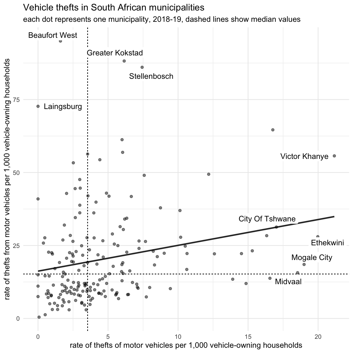
We can make some further changes to this chart. For example, instead of labelling areas on the plot we could label the municipalities with unusually high rates of vehicle theft. If we add too much text to the chart then the chart will become cluttered and the text may overlap, so we will probably need to choose between labelling municipalities with unusually high values and labelling the regions as in Figure 14.15. Which you choose is a judgement call for you to make based on what you think is most likely to be useful for a particular audience. Many audiences for crime analysis will be particularly interested in municipalities with unusually high values, so we will choose to label those.
If we labelled every dot directly using geom_label(), labels at their exact data positions could obscure the dots and overlap one another. The ggrepel package extends ggplot2 with geom_label_repel(), which automatically moves labels apart and draws connecting lines where necessary. This makes selected labels much easier to read on a crowded scatter plot.
To use it, we will create a new column in the data called label. This column will contain the municipality name for municipalities with high rates and NA for all other rows. We will then use the na.rm = TRUE argument to geom_label_repel() to tell the function to ignore the deliberately missing labels without producing a warning. We will also specify aes(label = label) to tell ggplot2 which column contains the text to display. The thresholds of 17 and 65 below were chosen to label a manageable number of municipalities with unusually high values; they are not the result of a formal statistical test for outliers.
Finally, we can add a trend line to the plot. We do this using the geom_smooth() function from ggplot2. geom_smooth() can add different types of trend line to a plot, but in this example we will specify a simple linear trend line by setting method = "lm" (‘lm’ stands for linear model). We will also specify formula = y ~ x (the default) to avoid geom_smooth() producing a message to tell us what formula it used to calculate the trend. By default, geom_smooth() also adds a shaded uncertainty interval around the line. Statistical inference is outside the scope of this course, so we set se = FALSE to omit that interval.
Add this code to the chapter_14d.R file and run it.
The theft_of and theft_from columns control the position of every layer, so we map them to x and y in the main call to aes(). Only the label layer needs the label column, so we map it inside geom_label_repel(). If we mapped label in the main call, geom_smooth() would inherit an aesthetic it cannot use and would produce a warning.
From this chart, we can see which municipalities have particularly unusual vehicle-theft rates. For example, we might well want to explore the rates of theft from vehicles in Beaufort West or Stellenbosch municipalities to see what makes them so different from the others, and similarly for the rate of theft of vehicles in Ethekwini.
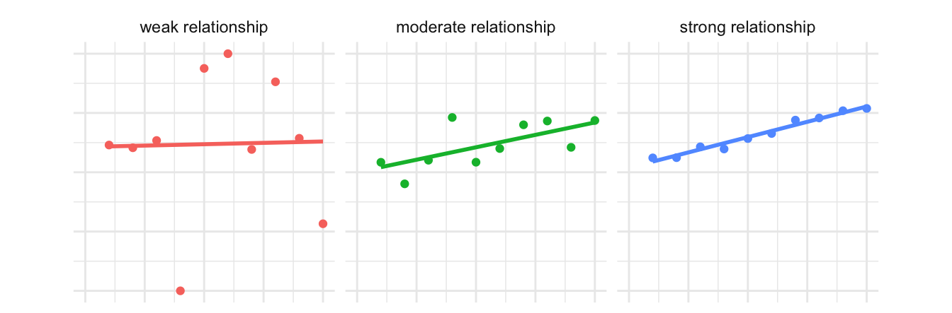
One note of caution when using geom_smooth(): this function will show the direction of the estimated relationship between two variables even when that relationship is weak. A trend line can also be strongly influenced by unusual observations or fail to represent a relationship that is not approximately linear.
For example, geom_smooth() produces a line showing the direction of the relationship between the two variables in each of these three charts, even though the relationship on the right is much stronger than the one on the left.
Be very careful about trying to interpret the strength of a relationship from the slope of a trend line. A correlation coefficient can summarise the strength of a linear relationship, while statistical inference can help quantify uncertainty, but those techniques and their assumptions are outside the scope of this course. For now, inspect the spread and shape of the points as well as the line, and avoid making claims that the chart cannot support.
Save chapter_14d.R by pressing . Your complete scatter-plot script should now look like this:
To check that the analysis is reproducible, restart R using the Restart R (⟳) button in Positron’s Console panel, then run the script from beginning to end.
In summary
In this chapter we have learned how to present data about crime at places without using maps. These techniques give us more flexibility about how to best present data to communicate the main points that we want to get across.
Whether to use a map or a chart, and which type of map or chart to use, are design decisions for you to make. When you make these decisions, always remember that what is most important is that your audience understands your message. This makes it very important that you understand your audience.
We have practised how to:
- choose between a map, table or chart based on the question and audience;
- prepare long-format data for presentation in a wide table;
- format and label tables using the gt package;
- use
ggauto() to create a useful first version of a chart;
- build a visualisation from
ggplot(), aesthetic mappings and geoms;
- use geoms, labels and themes in a ggplot2 stack;
- create clear bar charts and order their categories by value;
- use accessible colour palettes and check charts for common colour-vision differences;
- visualise distributions with raincloud plots and ridge plots; and
- compare two numeric variables using an annotated scatter plot.
Visualising data with charts is a very large topic and there are lots of resources available to help you learn more. To get started, you might want to look at:
Answer these questions to check you have understood the main points covered in this chapter. Write between 50 and 100 words to answer each question.
- Explain at least two scenarios where using a table or a chart would be more effective than a map for presenting spatial data.
- What is
ggauto() useful for, and why might you subsequently choose to rebuild its output using ggplot() and a geom_*() function?
- Explain the difference between mapping a column to an aesthetic inside
aes() and setting an aesthetic to a constant value inside a geom_*() function.
- How do raincloud plots and ridge plots represent distributions, and what should you consider when deciding which is suitable for an audience?
- Why should you check how a chart appears to people with different colour vision, and how can you do this in R?
- How can median lines and selected non-overlapping labels help an audience interpret a scatter plot?